Case Study · LensHH-LT
Vignetting factors — and why we optimize the apertures instead
Lens designers often shrink the diameters of selected elements on purpose. There are two common reasons: to make the lens smaller and lighter, or to improve off-axis image quality. Either way, undersizing an element clips part of the off-axis ray bundle — this is vignetting. This case study explains what vignetting and the vignetting factors that model it actually are, why they are awkward to carry through a global optimization, and how LensHH-LT sidesteps the problem by optimizing the physical apertures directly. The worked example at the end uses vignetting to improve off-axis performance.
What vignetting is
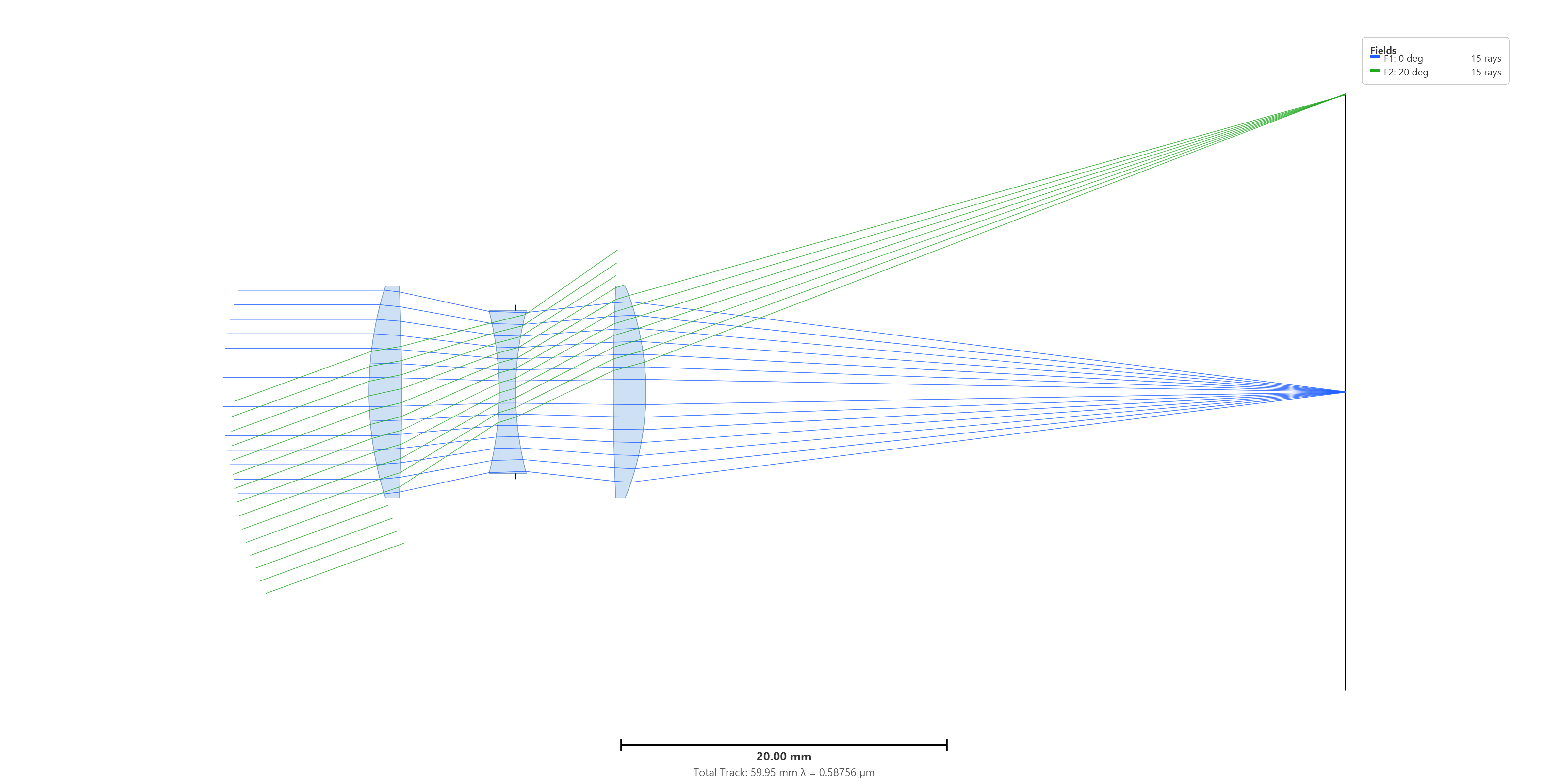
At every iteration of an optimization, a lens design code computes the diameter each surface would need in order to pass all the rays coming from the entrance pupil. Wherever the designer has fixed a diameter smaller than that computed value, some rays no longer make it through. For an off-axis field point, that clips the cone reaching the image, which raises the effective F/# and dims the edge of the field — a drop in relative illumination.
Why accept that? Two reasons. The first is size and weight: trimming the outer elements makes a smaller, lighter lens. The second is image quality: the rays at the edge of the pupil are often the most aberrated, so removing them can sharpen the off-axis image. The trade is straightforward to state — the designer gives up some edge illumination in exchange for a smaller lens or better off-axis performance. (One caution: if a diameter is reduced so far that it also clips the on-axis cone, that surface has quietly become the aperture stop of the system — almost never the intent.)
The vignetted pupil is a “cat’s eye”
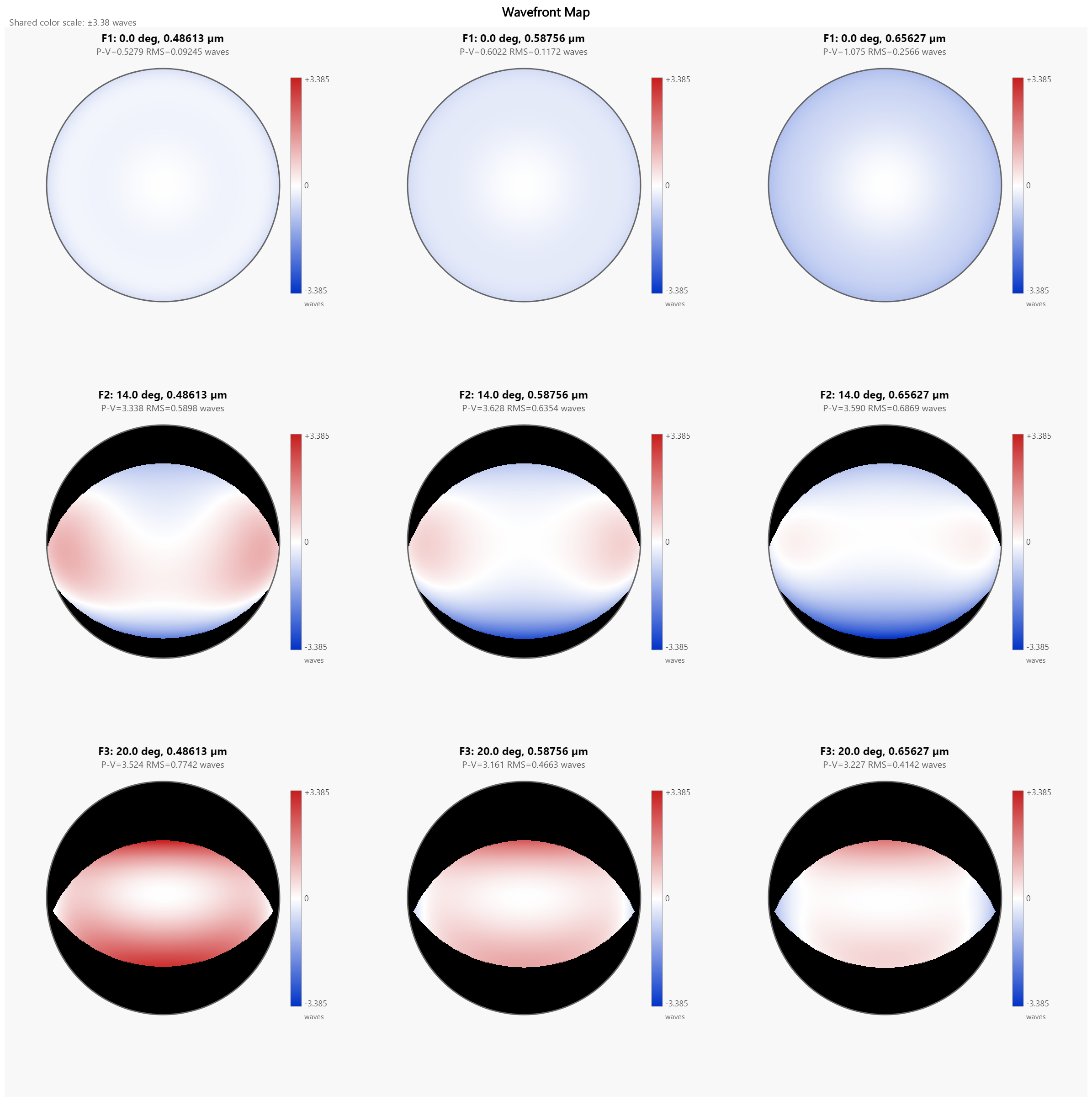
Look at an off-axis field through the entrance pupil and the surviving region is no longer a full circle. Each element aperture projects to a circle in pupil coordinates, and off-axis those circles are shifted relative to one another; the part of the pupil that actually passes through the system is their overlap — a lens-shaped region commonly called a “cat’s eye.” In the wavefront map below, the on-axis field (top row) fills the pupil, while the 20° field (bottom row) shows the cat’s eye, with the clipped regions in black.
What vignetting factors are
Here is the practical problem the factors solve. If the optimizer launched a grid of rays across the full circular pupil, most of them would land in the black region at an off-axis field and fail to trace. The few that survive give a noisy, unreliable spot-size estimate. You could fix that by sampling the pupil far more densely, but a denser grid makes every merit-function evaluation much slower — and an optimizer evaluates the merit thousands of times.
Vignetting factors are the standard workaround. The surviving region of the pupil is fitted with an ellipse, and during ray tracing the normalized pupil coordinates are remapped so that the sampling grid lands inside that ellipse instead of the full circle. Two numbers shift the ellipse’s center and two compress its width and height:
Px′ = VDX + Px · (1 − VCX)Py′ = VDY + Py · (1 − VCY)
VDX, VDY re-center the sampling on the vignetted pupil;
VCX, VCY shrink it to fit. The remapped points don’t need to
match the true boundary exactly — the goal is simply to keep most rays
inside the region that actually passes through the system. With the factors on, a
sparse, fast grid samples the surviving pupil well enough to give an accurate spot
size, so the merit function stays both cheap and honest.
When they’re computed — and why global optimization is hard
The factors are usually computed once, before optimization begins, from the starting design. For local optimization, where the design barely moves, that is fine. Global optimization is the hard case: the search may start far from the final form, and that final form may need vignetting to meet the specification at all. The vignetted pupil you are trying to reach doesn’t exist yet, so factors frozen at the start describe the wrong design. As the optimizer reshapes the lens, the true vignetting drifts away from the frozen factors; rays that have become vignetted are simply discarded, and a metric like RMS spot size can even appear to increase after a run meant to reduce it, because the set of rays being averaged changed underneath it.
Some codes respond by letting the vignetting factors themselves be optimization variables. The difficulty is that the factors are an abstraction of the pupil, not a physical quantity: there is no guarantee the values an optimizer settles on correspond to a set of clear-aperture diameters any real lens would produce. It then falls to the designer to check, after the fact, that the final diameters actually reproduce those factors — and if they don’t, the result isn’t realizable.
The LensHH-LT approach: vary the diameters
LensHH-LT takes the other route on both counts. Rather than exposing the vignetting factors, it lets you set the clear-aperture semi-diameter of any surface as a variable. The semi-diameters are the physical quantities, so optimizing them keeps the design in the realizable space by construction — whatever the optimizer arrives at is, by definition, buildable. The vignetting factors, when enabled, are internal to the engine and are recomputed automatically every time the merit function is evaluated, right after the semi-diameters update. They are always current, and the designer never edits them by hand. When you want the un-approximated truth for a finished design, clear the factors and evaluate a dense grid.
A worked example: improving off-axis performance
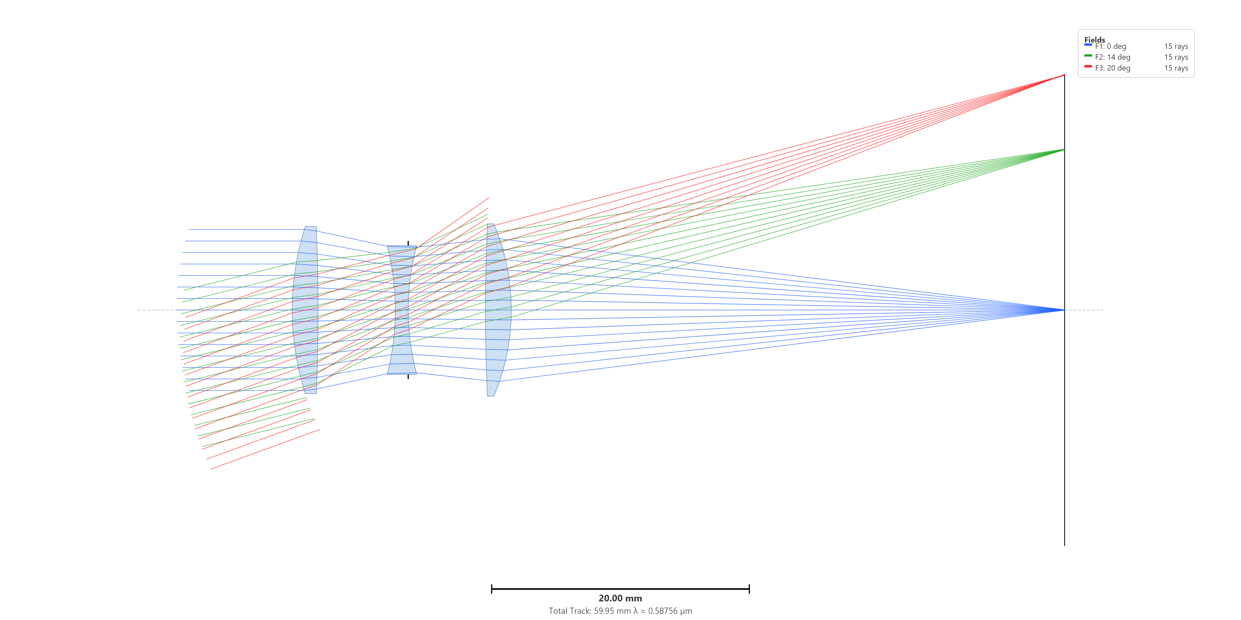
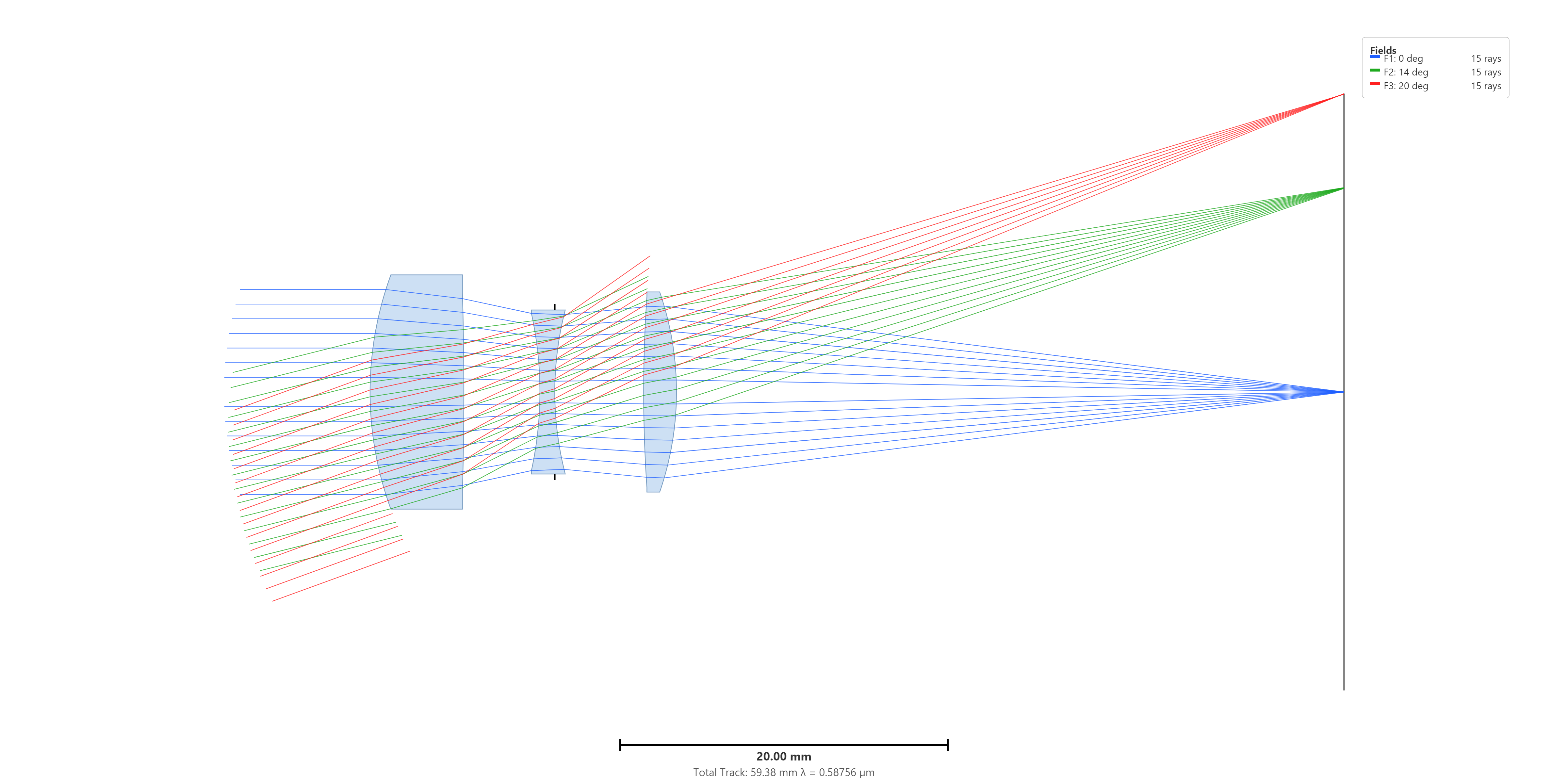
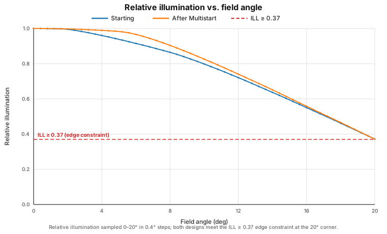
This example uses vignetting for the second reason — better off-axis image quality, not a smaller lens. The design is a Cooke triplet: 12.5 mm entrance pupil, 50 mm focal length (f/4), over a ±20° field, at the F, d and C lines. It vignettes to control its off-axis aberrations, so the edge of the field is dim — relative illumination is about 37% at 20°. The merit function accepts that vignetting but bounds it: an illumination operand holds the 20° field at or above 37%, alongside the focal length, edge- and center-thickness constraints, an on-axis RMS spot term, and a lateral-color term at the edge.
The variables are the curvatures and thicknesses of all three elements, glass substitution on the outer elements and the flint, and — the point of the exercise — the Fixed clear-aperture semi-diameters of the two outer elements, S1 (front) and S5 (rear). A Multistart run reduced the merit from 0.303 to 2.88×10⁻³. The two aperture variables moved in opposite directions: the front semi-diameter grew from 6.50 to 7.14, the rear shrank from 6.50 to 5.83 — an asymmetric split that started from symmetric 6.50 apertures. The glasses swapped from SK16 to N-SK16 on the outer elements and from F4 to SF2 on the flint.
The vignetting ellipse tracked the apertures
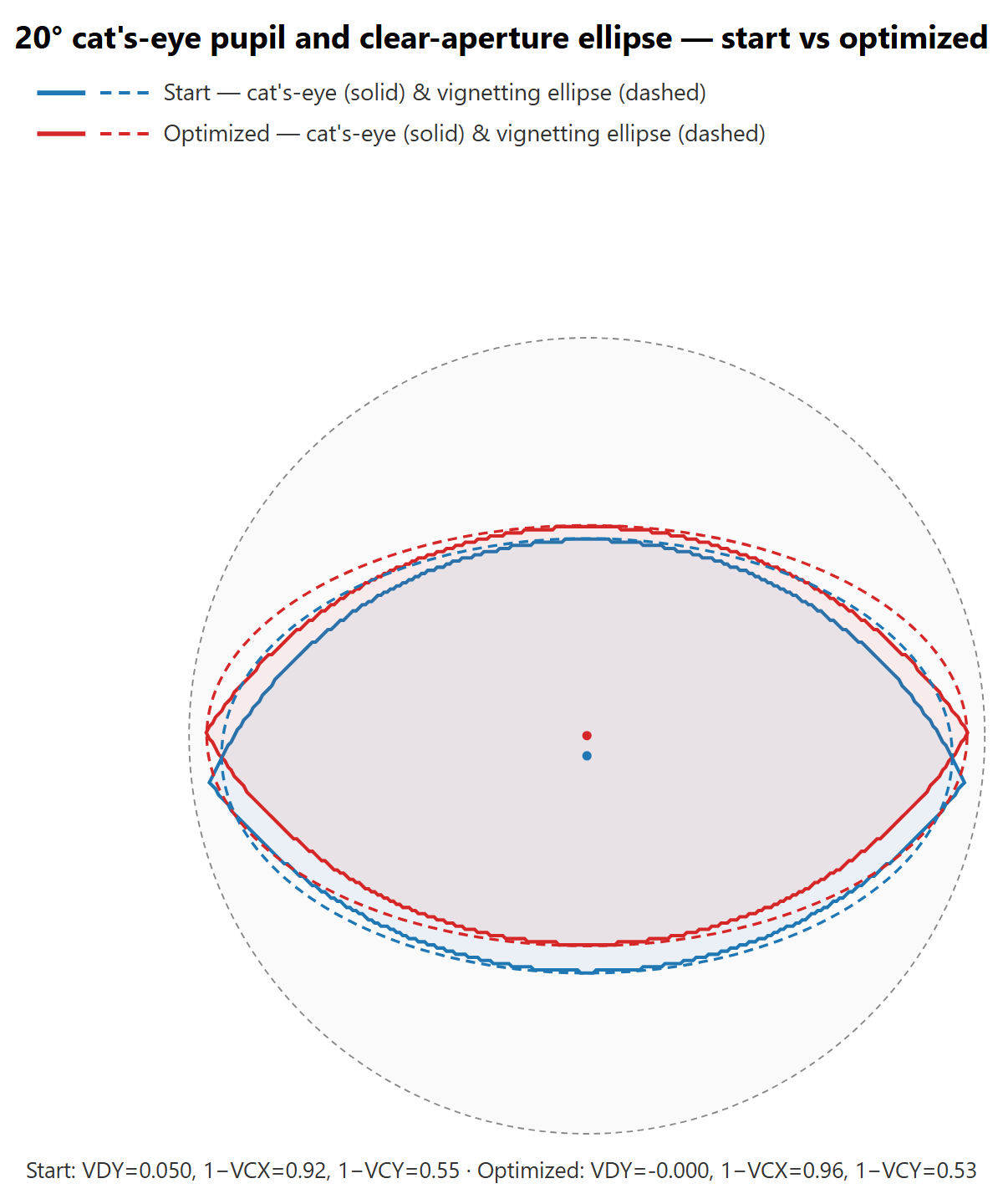
Because the semi-diameters were the variables, the ellipse the engine fits to the surviving pupil moved with them. At the 20° field the starting ellipse (blue) sits slightly high — its center above the pupil axis, because the symmetric apertures clip the off-axis cone unevenly. After optimization the ellipse (red) re-centers and widens, tracking the new front-larger / rear-smaller split, while the surviving pupil area — and thus the ~37% edge illumination — is essentially unchanged. The designer never touched the ellipse; it followed the apertures, staying consistent with the design at every trial.
Layout
Spot diagram (64×64 grid, using vignetting factors)
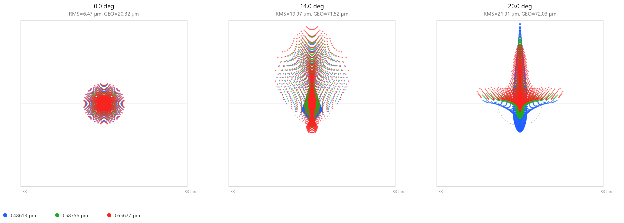
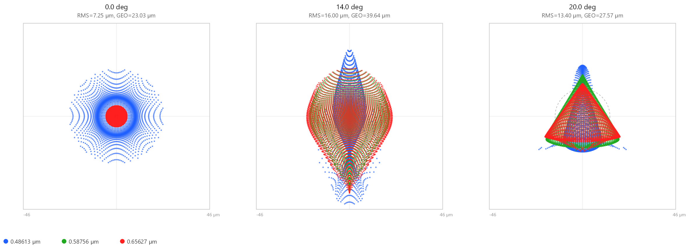
Spot size (µm)
| Field | RMS before | RMS after | GEO before | GEO after |
|---|---|---|---|---|
| 0° | 6.47 | 7.25 | 20.32 | 23.03 |
| 14° | 19.97 | 16.00 | 71.52 | 39.64 |
| 20° | 21.91 | 13.42 | 72.03 | 27.57 |
Off-axis imaging improves substantially — the 20° RMS spot drops ~39% and the worst-ray (geometric) extent falls by more than half — at the cost of a small increase in the on-axis spot, the expected trade for balancing the field.
Relative illumination
What’s worth taking away
- Vignetting is a deliberate trade. Undersizing elements dims the edge of the field, in exchange for a smaller lens or sharper off-axis imaging.
- Vignetting factors are a sampling aid, not physics. They remap pupil sampling onto the surviving cat’s-eye so a sparse, fast grid stays accurate — which is exactly why treating them as free variables can drift away from any realizable set of diameters.
- Vary the physical quantity, and keep it current. Optimizing the semi-diameters keeps every trial buildable, and recomputing the factors each merit evaluation keeps the vignetting model matched to the current design.
Run this yourself
Set any surface’s semi-diameter as a variable in the Lens Editor, add an illumination operand to bound the edge, and run Multistart — the vignetting factors update themselves as the apertures move.
Download free trial Back to LensHH-LT