Overview
LensHH-LT is a sequential optical-design tool for refractive and reflective imaging systems — triplets, Petzvals, double Gauss, Schmidt-Cassegrain and Maksutov telescopes, and similar designs.
Load a starting design from ZEMAX (.zmx), OSLO (.len), Optalix
(.otx), Code V (.seq), Optiland (.json), or LensHH-LT's native
.lhlt; explore it
through a full set of polychromatic analyses (spot, MTF, wavefront,
ray and OPD fans, Seidel, Zernike, distortion, field curvature,
relative illumination, chromatic focal shift); and refine it with
merit-function-driven optimization (Levenberg-Marquardt, multistart,
basin hopping) plus design-shape operators (split-element,
SPC synthesis) and per-element glass substitution.
The same engine is reachable from a C# API, an interactive CLI, and an MCP server for LLM agents (Claude Code, Cursor, etc.). The desktop app runs on Windows, macOS, and Linux.
This guide walks through the GUI, every analysis panel, every merit-function operand, the optimizers, the glass-catalog system, and the programmatic interfaces.
Pages
- Getting Started — install, open a sample lens, run a first analysis, run a first optimization.
- Analyses Reference — every analysis panel (spot, MTF, wavefront, ray fans, Seidel, Zernike, etc.) with inputs and interpretation tips.
- Merit Function Reference — every merit function operand with its inputs, meaning, and typical usage.
- Optimization — the optimizers (Local LM, Multistart, Global Search, Basin Hopping) plus design-shape operators (split-element, SPC synthesis), and when to use each.
- Semi-Diameter as an Optimization Variable — make a Fixed-aperture surface's clear-aperture semi-diameter a variable and let the optimizer size the aperture directly; worked Cooke-triplet-with-vignetting case study.
- Automatic Vignetting Factors — sample the vignetted pupil correctly for off-axis fields in analysis and optimization; recalculated automatically as the apertures change.
- GPU Acceleration — configure the GPU options in Preferences and confirm they're running with the live GPU status chip; which optimizers use the GPU and which don't.
- Glass Catalogs — AGF format, the five shipping catalogs, preference order, custom catalogs via GlassCatalogGenerator, and glass substitution during optimization.
- API, CLI, and MCP — programmatic access: embed the C# API in your own .NET code, drive the engine from the interactive CLI, or expose it to Claude/Cursor/other MCP hosts.
- Agent Workflow — Stock-Lens-Based Design —
recipe for an LLM agent to chain
search_stock_lenses→insert_stock_lens→ analyze →reverse_lens→ optimize against the bundled 7,600-part Edmund + Thorlabs + Ross Optical catalog. - Sasian Design — Stock-Lens Triplet Pipeline —
end-to-end MCP orchestrator (
sasian_design_start/_status/_cancel/_discard) that builds a Cooke-triplet skeleton, free-optimizes with glass substitution, then walks element-by-element replacing each free-form singlet with the best matching catalog stock part. Phase 2 entry for doublet retrofits. - Building from Source — optional on every platform (Windows installer, pre-signed macOS zip package, Linux AppImage all ship with each release); for users tracking main.
Scope
LensHH-LT supports the common workflow of a general-purpose lens designer:
- Loading lens files from ZEMAX (
.zmx), OSLO (.len), Optalix (.otx), Code V (.seq), Optiland (.json), or LensHH-LT's native.lhlt. - Standard and Even Asphere surfaces.
- EPD or F/# apertures, object-angle or object-height fields.
- Polychromatic spot, PSF, and MTF analyses (wavefront, OPD, Zernike, and Seidel are evaluated one wavelength at a time).
- Merit-function-driven optimization with variables and pickups.
- Glass catalogs in AGF format (five catalogs ship with the installer).
It does not handle configurations, coatings, thermal/environmental effects, tolerancing data, tilts and decenters, folds, or non-standard surface types. For those, see the full LensHH product.
Feedback
File issues or suggestions at the project's GitHub repository.
Getting Started
Install (Windows)
- Run
LensHH-LT-Setup-<version>.exe. - If the installer warns that .NET 8.0 Desktop Runtime is missing, accept the prompt to download it from Microsoft, install, then re-run the LensHH-LT installer.
- Launch LensHH-LT from the Start Menu.
Sample lens files are installed under <install>\samples\ with the
.lhlt extension.
Install (macOS, Apple Silicon)
macOS builds ship as a zip archive — LensHH-LT-osx-arm64-<version>.zip
in the release downloads — containing the GUI, CLI, MCP server, Ollama
bridge, and benchmarking tool, plus the full sample-lens set, the
stock-lens catalog, and the documentation. All binaries are pre-signed;
there is no codesign step.
Unzip (double-click in Finder), then open Terminal in the unzipped folder.
Run the two first-run commands (also listed in the bundled
README-macOS.txt):xattr -dr com.apple.quarantine . chmod +x app/LensHH.App cli/LensHH.CLI mcp/LensHH.Mcp \ renderapp/LensHH.RenderApp ollama/LensHH.OllamaBridge \ bench/MeritEvalBenchThe first clears the download-quarantine flag (macOS's equivalent of SmartScreen "Run anyway"); the second restores the Unix execute bits, which a zip archive built on Windows doesn't carry.
Launch the GUI:
cd app && ./LensHH.App
Samples are in samples/, and the User Guide PDF plus searchable HTML
help are in docs/. Keep the package folder structure intact — the
tools locate the shared stock-lens catalog relative to their own
folders.
Requirements and limits:
- Apple Silicon (M1 or later) only. Intel Macs are not supported — the native ray-trace library ships arm64-only.
- No GPU acceleration on macOS — optimization runs on the CPU.
- If macOS still refuses to open a binary: System Settings → Privacy & Security → scroll to the blocked item → Open Anyway.
License & Trial
LensHH-LT is distributed under a hybrid license:
- Source code (GUI, CLI, MCP server, public C# API, IO, rendering, configurators) is open source under the MIT license. Fork it, modify it, redistribute it.
- Optical engine binaries (
engine/LensHH.Core.dllplus the platform-specific native ray-trace libraries) are proprietary to Synapse Optics and require an activation token to run.
See LICENSE at the project root for the full terms.
Ray tracing, optimization, and analyses won't run until you've activated either a free trial or a paid license. Both flows live under the Help menu.
Start a free trial (45 days)
- Help → Start Free Trial...
- Enter your email address and click Send Code. A six-digit verification code is sent to that address.
- Enter the code in the dialog and click Activate.
- The trial runs for 45 days from activation. Help → License Status... shows the days remaining at any time.
One trial per email address. Reinstalling does not reset the clock.
If your network blocks the activation server
If your corporate firewall cannot reach the licensing host (see Network requirements below), use the offline path on the same dialog:
Help → Start Free Trial... → click Activate offline from token file... at the bottom of the dialog.
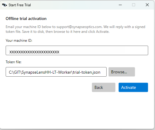
Email the machine ID shown in the dialog, plus the email address you'd like the trial bound to, to
support@synapseoptics.com.Synapse Optics replies with a signed
trial-token.jsonfile. Save it locally (USB transfer is fine — the machine doesn't need internet to receive the file).Back in the dialog, click Browse..., select the token file, and click Activate. The 45-day clock starts at activation.
The token is bound to the machine ID you sent — the embedded signature only verifies on that machine. The flow works on fully air-gapped machines.
Activate a paid license
- Help → Activate License...
- Paste your license key and click Activate. The dialog contacts the activation server, binds the seat to this machine, and stores a signed token locally — subsequent launches don't need network access.
- The Help menu's License Status... entry shows the active license and machine binding.
Move a license to another machine
A license is one seat. To free it up:
- On the current machine: Help → Deactivate This Machine... — re-enter your license key to confirm. The server frees the seat.
- On the new machine: Help → Activate License... with the same key.
Offline activation
If the new machine has no internet access, request an offline
activation token from your distributor (mention your machine ID,
shown under Help → License Status...), save it as a .json
file, and import it via Help → Activate License... — the dialog
detects a token file vs a key string automatically.
Network requirements
LensHH-LT only reaches the network for license activation and deactivation. Ray tracing, optimization, analyses, and file I/O run fully offline once activated.
If your IT department restricts outbound traffic, the values below are everything they need to whitelist:
| Field | Value |
|---|---|
| Hostname | synapseoptics-license.javier-ruiz.workers.dev |
| Protocol / port | HTTPS / TCP 443 |
| Methods | POST (trial request, trial verify, activate, deactivate) |
| Hosting | Cloudflare Workers (anycast — whitelist by hostname / SNI; no fixed IP range) |
| TLS | TLS 1.2 or 1.3, public CA-signed certificate |
| TLS inspection | Do not intercept — the client pins to the hostname's certificate via SNI |
| Direction | Outbound only — LensHH-LT does not accept inbound connections |
If the host cannot be allowlisted, both the offline trial and the offline paid-license activation flows work with zero network access on the target machine.
Your First Lens
File → Open… — point at any file in
<install>\samples\(tryCookeTriplet.lhltfor the classic three-element form, orHeliar.lhltfor a five-element triplet derivative).The main window opens on the Lens Editor — the lens prescription table. Tabs along the top switch between the Lens Editor, the 2D Layout, and the Merit Function editor.
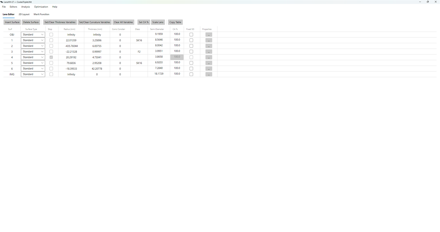
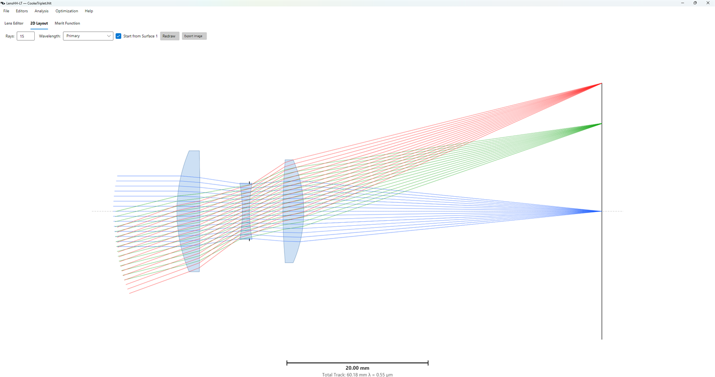
Click 2D Layout to see the design ray-traced:
Open a spot diagram: Analysis → Spot Diagram.
Open a wavefront map: Analysis → Wavefront Map.
Close both and try optimization — read on.
Reading the prescription table
Each row in the Lens Editor is one surface, ordered object → image:
| Column | What it is |
|---|---|
| Surf | Surface number (OBJ, then 1, 2, …, IMG). |
| Surface Type | Standard (spherical), an aspheric type, Paraxial (an ideal thin lens defined by a focal length), or ABCD (a ray-transfer-matrix black box) — see below. |
| Stop | Checkbox marking the aperture stop. |
| Radius (mm) | Radius of curvature (Infinity for a flat surface). |
| Thickness (mm) | Axial distance to the next surface. |
| Conic Constant | Conic k (0 = sphere). |
| Glass | Material of the space after the surface (blank = air). |
| Semi-Diameter | Clear-aperture radius — how it's set depends on Fixed SD. |
| CA % | Clear-aperture percent, on Auto surfaces (see below). |
| Fixed SD | Checkbox choosing how the semi-diameter is set. |
| Properties | The … button — per-surface variable / pickup, aspheric, and aperture settings. |
Paraxial (ideal thin lens) surfaces. Setting a surface's type to
Paraxial turns it into an ideal thin lens defined by a single focal
length (mm) — it bends rays with no aberration and no thickness. Radius,
conic, and glass are ignored and shown blank; the focal length is edited in the
surface Properties dialog (a positive f converges, negative diverges,
Infinity is afocal / no power). It carries the surrounding indices, so an
immersed ideal lens of focal length f in medium n focuses at n·f. Paraxial
surfaces are handy for representing a "perfect" element, a relay, or a stand-in
for a subsystem you have not designed yet. They run on CPU only (never the GPU),
and they are diffraction-limited: an on-axis WAVEX/OPD merit reads ≈ 0 at focus.
ABCD (ray-transfer-matrix) surfaces. An ABCD surface is a first-order
"black box" defined by four numbers — the paraxial ray-transfer matrix
[x'; ω'] = [[A, B], [C, D]] · [x; ω] acting on ray height x and geometric
slope ω (the same matrix applies in y). Like Paraxial, it has no radius,
conic, or glass — the four elements A, B, C, D are edited on the ABCD tab
of the surface Properties dialog, where each can be Fixed, Variable, or a
Pickup. The identity matrix (A = D = 1, B = C = 0) passes rays through
unchanged, which is the default for a new ABCD surface. It carries the
surrounding medium unchanged and contributes no aberration of its own.
ABCD surfaces are the tool for first-order synthesis: drop one (or several)
in as an ideal stand-in for a group you haven't designed, optimize the matrix
elements to meet your first-order and image-quality goals, then build real
lenses that reproduce the resulting matrices — using the A/B/C/D and
DET merit operands (see the Merit Function Reference) to
match a real group's matrix to the target. A lossless group in a single medium
has determinant A·D − B·C = 1, so constrain DET = 1 on each ABCD surface
to keep the optimized matrix physically realizable, and bound the elements
(especially C, the power) so the optimizer can't run them to infinity.
ABCD surfaces run on CPU only. Because a ray-transfer matrix carries no wavefront/phase information, analyses that require phase — OPD, MTF, Zernike, wavefront map — are unavailable while an ABCD surface is present; ray-based analyses (layout, spot, ray fan, distortion, Seidel, first-order) still work.
Apertures — the Semi-Diameter, CA %, and Fixed SD columns. These three work together to set each surface's clear aperture:
- Fixed SD unchecked (Auto — the default): LensHH re-solves the
semi-diameter from the traced ray bundle every time the design
changes, then scales it by that row's CA % (
100 %= the full bundle; a lower value stops the surface down, deliberately vignetting the margin). The Semi-Diameter cell is read-only in this mode — edit CA % instead. - Fixed SD checked (Fixed): you type the Semi-Diameter value directly and it's held regardless of the rays.
The stop is always Auto at 100 %, and the object row has no
aperture. The Set CA % button above the table applies a CA % — and
the Auto/Fixed mode — across a range of surfaces at once. Both the
semi-diameter (Fixed) and the CA % (Auto) can also be optimization
variables — see Aperture variables under Your First
Optimization, below.
Your First Optimization
The optimizer moves any parameter you've tagged Variable. Picking the right variable set is the central design decision; everything else (merit function, optimizer choice, bounds) just shapes the search. LensHH-LT gives you three ways to mark variables — pick whichever matches the granularity you need.
Marking variables
1. Bulk: thickness or curvature across a surface range
The fastest way to start. Above the Lens Editor table:
Set/Clear Thickness Variables opens a dialog with
Surface 1,Surface 2, and a Set / Clear radio. Click Set, choose a range (e.g. surfaces 1 through 6 to vary every glass and air thickness in the Cooke triplet), and OK. Every thickness in the range is now a variable.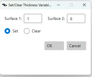
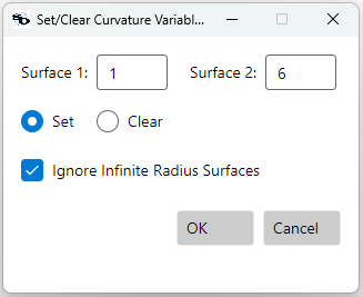
Set/Clear Curvature Variables is the same idea for curvatures. An extra checkbox Ignore Infinite Radius Surfaces keeps flat surfaces fixed (you almost always want this on).
Set/Clear Surface Parameter Variables does the same for the parameters of the special surface types. Choose a Surface Type (Even Asphere, Paraxial, or ABCD) and a Parameter — an aspheric coefficient
A2…A16, a Paraxial focal length (Diopters), or an ABCD elementA/B/C/D— then a surface range and Set / Clear. It applies to every surface of that type in the range, so you can, say, make theAelement a variable on all your ABCD surfaces in one action. It only sets or clears the variable flag (no bounds — set those in the Variable Editor).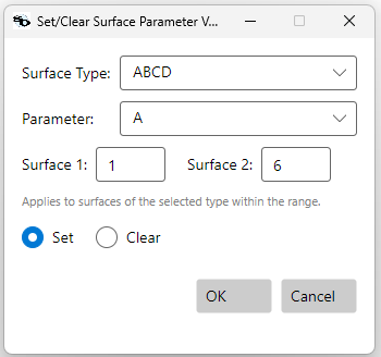
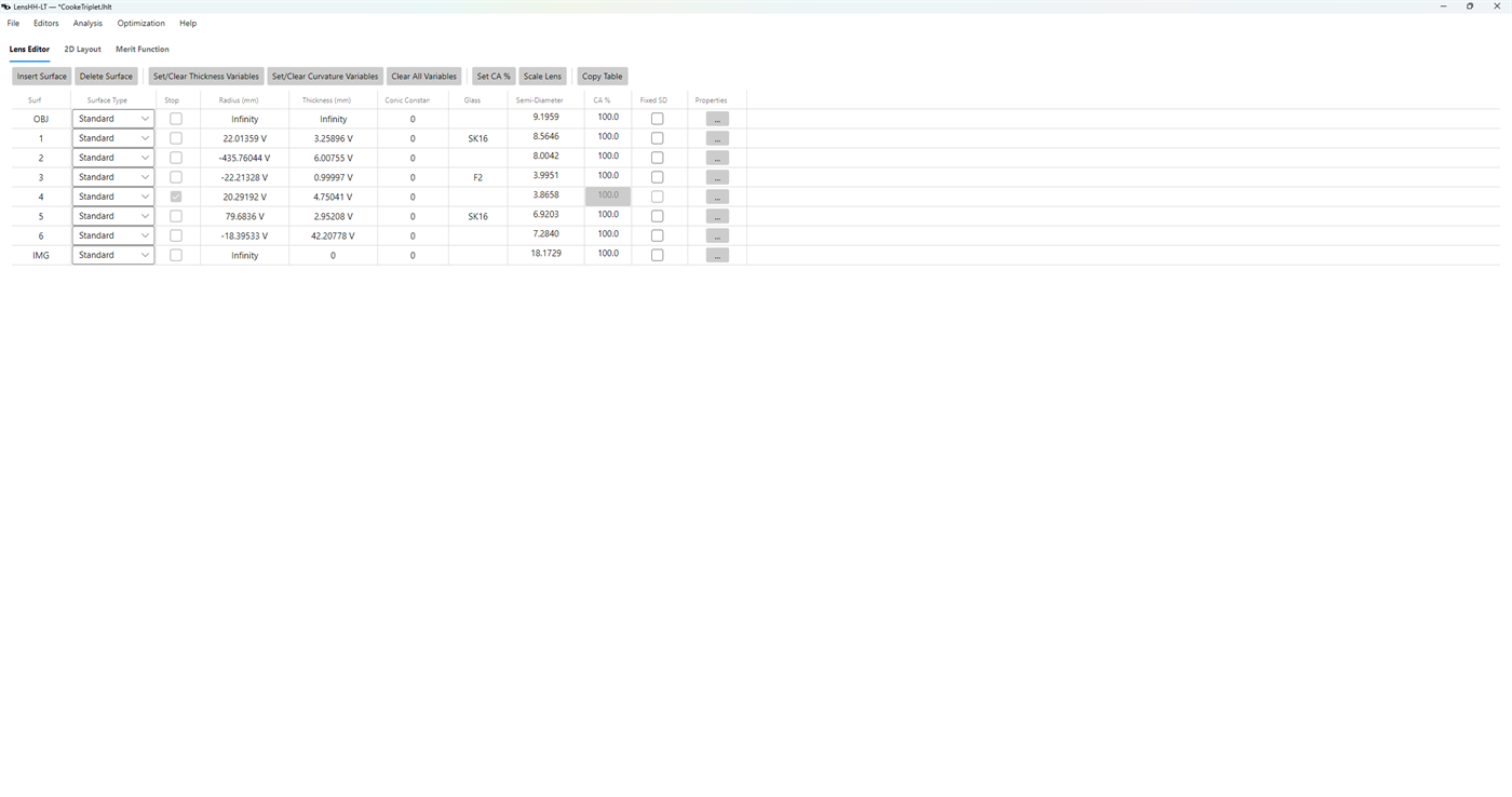
Each tagged parameter shows a V indicator next to its value in the Lens Editor table:
2. Per-surface fine-grained: the Properties dialog
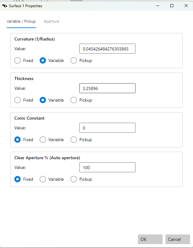
For one surface at a time, click the ... Properties button in
that surface's row. The Variable / Pickup tab has a section for
each of Curvature, Thickness, and Conic with three radio
buttons:
- Fixed — the optimizer leaves this parameter alone.
- Variable — the optimizer is free to change it.
- Pickup — the parameter is computed from another surface's
parameter as
Source × Scale + Offset. Use a pickup to lock two curvatures together (e.g., a symmetric singlet) or to drive an airspace from a glass thickness.
Choose Variable to mark the parameter as free.
3. Aspheric coefficients
On surfaces with aspheric type, the Properties dialog's Aspheric
tab lists every coefficient (A2 through A16) with a per-row
Var checkbox. Tick the ones you want optimized.
4. Aperture variables: semi-diameter and clear-aperture %
Recall from Reading the prescription table (above) that each surface's aperture is either Auto — a ray-traced semi-diameter scaled by its CA % — or Fixed — an explicit semi-diameter — chosen by the Fixed SD checkbox. Either of those quantities can be handed to the optimizer as a variable.
Making the aperture a variable — to adjust vignetting. The clear aperture is exactly what clips off-axis rays, so it is the knob that controls vignetting and relative illumination. You can hand that knob to the optimizer:
- in Auto mode, mark the surface's CA % as a variable;
- in Fixed mode, mark its semi-diameter as a variable.
Both are set on the Properties dialog's Variable / Pickup tab, the
same way as curvature or thickness (a V marker then appears next to
the value in the Lens Editor). The stop surface is the one
exception: its semi-diameter is the system aperture (fixed by the
EPD / F‑number / NA), so it can never be an aperture variable — the
Variable option is disabled for it, and the optimizer ignores the
flag even if a loaded file sets it. The optimizer can now open or stop
down each non-stop surface's aperture to trade image quality against
vignetting —
for instance widening an aperture that was clipping the off-axis
bundle. Pair an aperture variable with a dense rectangular
spot/wavefront grid (see Rectangular operands in
merit-function.md) so the merit's response to the
moving pupil edge stays smooth.
Always bound an aperture variable. Unlike a curvature, a CA % or semi-diameter has no natural restoring force — left unconstrained, the optimizer will happily drive it to zero (closing the surface) or to an absurd value if that shaves the merit. Give it a Min/Max constraint in the Variable Editor (next section) — for example hold CA % between ~85 % and 100 %, or keep a Fixed semi-diameter inside the element's real mechanical range.
Setting bounds (Min/Max constraints)
Bounds live under Optimization → Variable Editor — not on the Lens Editor table. Open it after you've marked your variables and the dialog lists every variable as a row:
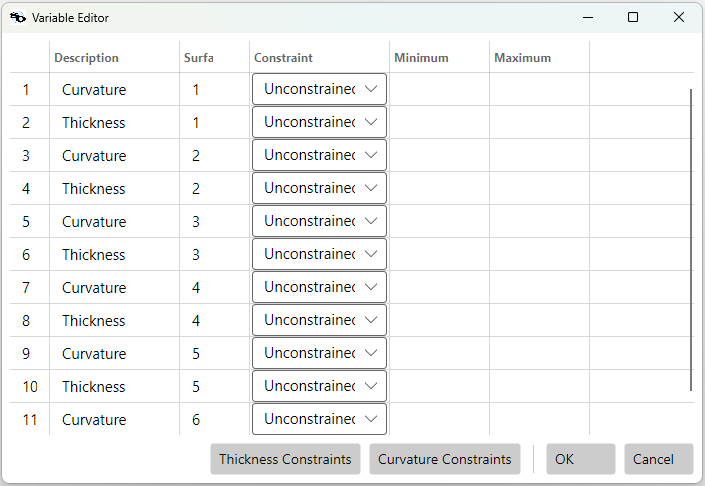
Each row shows:
| Column | Meaning |
|---|---|
| # | Variable number. |
| Description | What the variable is (e.g. Curvature, Thickness). |
| Surf | The surface index it lives on. |
| Constraint | A combo: Unconstrained, Min, Max, or Min/Max. |
| Minimum | Lower bound. Used if Constraint is Min or Min/Max. |
| Maximum | Upper bound. Used if Constraint is Max or Min/Max. |
Inside the optimizer, bounds are enforced via an unbounded parameter transformation, so the LM solver never tries an illegal value — it just slows down near the wall.
For broad ranges, the Thickness Constraints and Curvature
Constraints buttons at the bottom of the Variable Editor open a
bulk dialog. The thickness one is especially useful — pick a
surface range, an All / Glass / Air selector, a Constraint
mode, and a single Min / Max pair, and the dialog applies them
to every matching thickness variable in the range. Run it twice to
get separate glass and air rules:
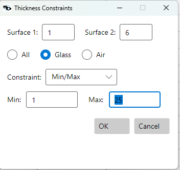
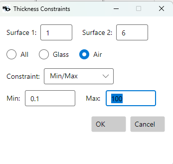
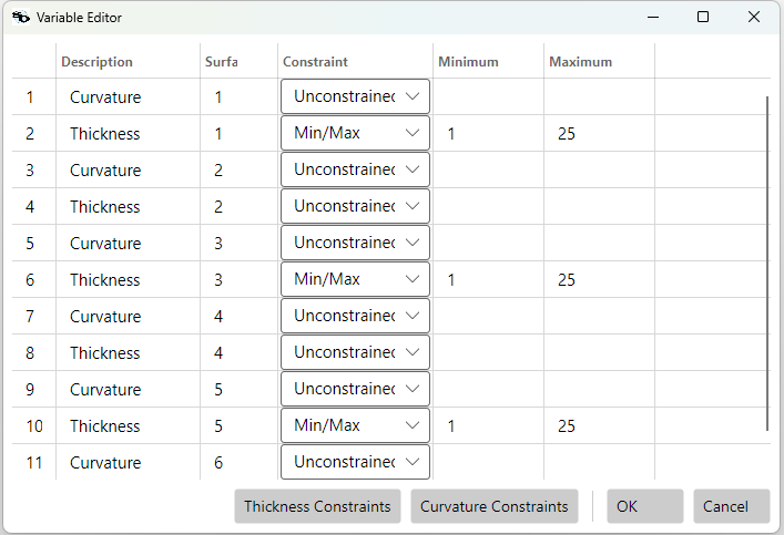
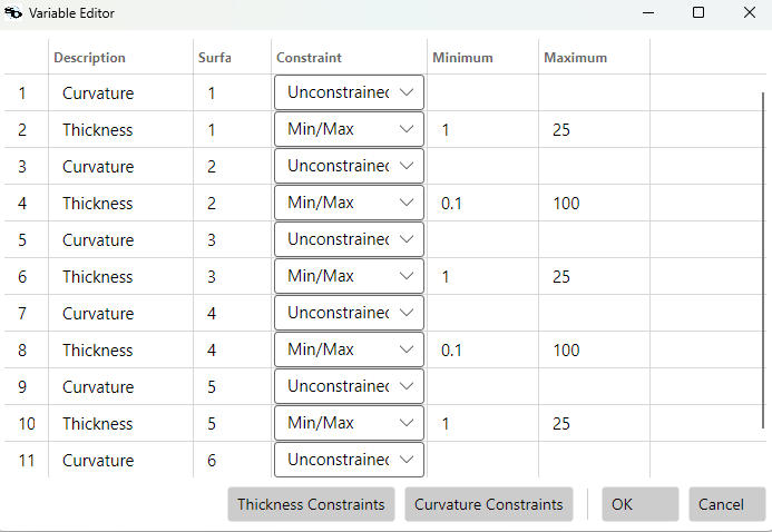
After both runs the Variable Editor reflects the populated
constraints — glass thicknesses bounded [1, 25] mm, air gaps
bounded [0.1, 100] mm:
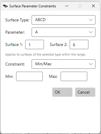
A third button, Surface Parameter Constraints, does the same for
the parameters of the special surface types. Pick a Surface Type
(Even Asphere, Paraxial, or ABCD) and a Parameter (an aspheric
coefficient, the Paraxial diopters, or an ABCD A/B/C/D element), a
surface range, a Constraint mode, and a Min / Max pair — the
dialog sets that parameter as a variable with the chosen bounds on
every surface of that type in the range. It's the one-step way to, for
example, make every ABCD C element a variable bounded to a realizable
power range across a whole synthesis stack.
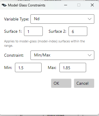
A fourth button, Model Glass Constraint, does the same for the
model-glass (fictitious-glass) parameters. Pick a Variable Type —
Nd (refractive index), Vd (Abbe number), or dPgF (partial-dispersion
deviation) — a surface range, a Constraint mode, and a Min / Max
pair, and the dialog sets that parameter as a variable with the chosen
bounds on every qualifying surface in the range. It applies only to
surfaces already in model-index mode — a real catalog glass has no
Nd/Vd/dPgF to vary, so it is skipped rather than converted. This is
the one-step way to turn a stack of model glasses loose inside a
manufacturable index / Abbe / partial-dispersion box before you substitute
real catalog glasses (see Glass catalogs for how model
glasses and substitution work):
Building a merit function
Optimization → Merit Function. Add operands via the Insert button. A good starting merit function has three layers; cutting any of them risks an unphysical or shallow-converged design.
A note on composite operands.
WAVEX,SPOT,WAVEM, and the other image-quality operands are composite: a single row evaluates over every field point and every wavelength in the system at once. You don't pickHx/HyorWavefor these — the operand automatically applies the per-field weights from the Field editor and the per-wavelength weights from the Wavelength editor as internal sub-weights (the engine multipliesmacro_weight × field_weight × wavelength_weight × pupil_weightfor each hidden expanded operand). OneWAVEXrow covers the whole field × wavelength × pupil grid, so you don't need a long merit function with many rows to control image quality.
Reading the merit grid:
Modeand the two bound columns. The Merit Function table doesn't have separateMinandMaxcolumns. It hasBound 1andBound 2, and how they're interpreted depends on theModecombo on the same row:
ModeBound 1is...Bound 2is...Targetthe target value (hidden, not used) Minthe minimum value (hidden) Maxthe maximum value (hidden) Min/Maxthe minimum value the maximum value Note that
Maxmode puts the upper bound inBound 1, notBound 2—Bound 2is only visible/editable whenMode = Min/Max. When the example rows further down say "min=..." and "max=..." together, setMode = Min/Maxand put the min inBound 1and the max inBound 2. When an example shows just "target=...", setMode = Targetand put the value inBound 1.
What
ValueandErrormean in each row. The two read-only columns at the right of every operand show:
Value— what the operand currently evaluates to in the live design (e.g. forEFL, the focal length in mm; forEGover a surface span, the worst edge thickness; see "Span operands" below).
Error— the row's residual contribution. The LM solver minimizesΣ Error²across the whole table.Erroris always(value − reference) × weight, where the reference depends onMode:
ModeError(residual)Target(value − target) × weight. Always nonzero unlessvalue == target.Min(value − min) × weightifvalue < min, else 0. One-sided deadband.Max(value − max) × weightifvalue > max, else 0. One-sided deadband.Min/Max(value − min) × weightif belowmin;(value − max) × weightif abovemax; else 0. Two-sided deadband.A row whose
Valueis inside its bounds showsError = 0— it contributes nothing to the merit and acts purely as a guardrail ("don't go past this"). That's why boundary operands (EG,CTG, etc.) don't fight image quality while the design stays well-formed.Span operands (
Surface≠Surface2). When the row covers a surface range, the operand evaluates the underlying parameter (center thickness, edge thickness, semi-diameter, etc.) at every surface in the span and tracks the per-span minimum and maximum. The displayedValuethen represents the span as one number, chosen so the residual reflects the worst violation:
- Min violated (any surface in the span has value below
Min):Valueis the smallest value across the span — the worst-offending surface.- Max violated:
Valueis the largest value across the span.- Both violated:
Valueis whichever side has the larger gap from its bound (the more critical violation).- All satisfied:
Valueis the smaller of the two extremes (closest to the lower constraint), so you can read how much margin the worst surface still has.Targetmode:Valueis the mid-point(minVal + maxVal) / 2of the span.One row → one residual, no matter how many surfaces violate. A span operand produces exactly one residual per evaluation, computed from the single worst-offending surface in the span. Multiple violators do not add together. If three surfaces in the span have edge thicknesses
0.1,0.3,0.4andMin = 0.5, the row'sErroris(0.1 − 0.5) × weight— driven by the0.1surface alone; the other two contribute zero.In practice the optimizer resolves multi-surface violations iteratively: it fixes the worst surface this iteration, the next-worst becomes the new worst, and so on across iterations. This is normally what you want — it keeps geometric-bound rows from drowning out image quality just because the design happens to have many elements.
If you want additive behavior — every violator contributing independently to
Σ Error²— write one row per surface (setSurface = Surface2to a single index, repeat for each surface). You lose the auto-protection benefit when surfaces get inserted later, but each violation enters the merit on its own. A common hybrid: keep the span row for blanket protection and add a per-surface row for any surface you know is marginal (e.g., the one closest to the stop on a fast lens). Both contribute, so the marginal surface gets extra optimizer attention without losing the span coverage.Adding a new surface during design — split-element, doublet insertion — automatically becomes part of the span row's evaluation, so structural edits stay protected without merit- function maintenance.
1. Image quality
Recommended: WAVEX — RMS wavefront error in waves, with piston
and tilt removed. Wavefront error is what diffraction-quality images
actually care about, and the LM solver converges on it more reliably
than on transverse ray aberration. Set Rings = 6, Arms = 12,
Weight = 1. That's it — no field or wavelength specifiers, because
WAVEX already integrates over both.
SPOT (RMS spot size) is also composite and also tempting because
the units (mm) feel intuitive, but it's a poorer proxy for image
quality near the diffraction limit and tends to leave the optimizer
stuck in shallow local minima. Start with WAVEX unless your design
is many times the diffraction limit (where wavefront and spot stop
tracking each other).
2. First-order constraints
Lock the design's first-order properties so the optimizer doesn't trade them away for image quality:
EFL— locks focal length.Target = <desired EFL>,Weight = 100(see Weights — telling the optimizer what's paramount below for why).TTRACK(max total track),MAG(magnification),DITHETA(max F-θ distortion %), etc. — see the Merit Function Reference.
3. Physical-thickness boundaries (almost always required)
Without explicit constraints, the optimizer will gladly drive a lens to a vanishing center thickness or a negative edge thickness — both unphysical, both common failure modes. An effective optimization always enforces thickness boundaries.
The right tool depends on which thickness you're constraining:
Center thickness (the
Thicknessfield on a surface) is a single variable, so it's bounded most cleanly via variable bounds in the Variable Editor — see Setting bounds above. SetConstraint = Min and Maxon every glass-thickness variable, withMinimum ≈ 1 mmand a sensibleMaximum; same for every airspace, withMinimum ≈ 0.1 mm. The LM solver enforces these exactly through an unbounded parameter transformation, with no drag on convergence while the design is well-formed.Alternative — merit operands. Two operands cover the same ground for users who prefer to keep all geometric constraints in the merit function rather than split between Variable Editor and Merit Function:
CTG(Center Thickness for glass elements) andCTA(the air-gap analog). Both acceptSurface/Surface2spans andMin/Maxbounds. Either approach works — pick one and apply it consistently to every center thickness in the design; mixing and matching surface-by-surface is how holes get left.Edge thickness is a derived quantity (function of curvature and center thickness and semi-diameter), so it can't be expressed as a variable bound at all. You must use merit operands:
Operand Acts on Meaning EGGlass elements Edge thickness — set Min(andMax)EAAir gaps Edge thickness of an air space These are almost always necessary: a steeply-curved positive lens can have its edges cross zero even with a perfectly healthy center thickness. Set
Constraint = Min and Max,min = 0.5 mmfor glass,min = 0.1 mmfor air, and a sensible max so the optimizer doesn't run away.
Use surface spans, not individual surfaces.
EG,EA,CTG, andCTAall accept aSurfaceand aSurface2. Set them to the range of all optical surfaces (e.g.surface=1, surface2=6for a six-surface triplet) and a single row covers the whole lens. The benefit isn't just brevity: when you later split an element, add a doublet, or otherwise insert surfaces, the merit function automatically protects the new geometry too. A merit function that names individual surfaces becomes silently incomplete after every structural edit.
4. Weights — telling the optimizer what's paramount
The numbers in the Weight column are how you express priority to
the optimizer. The LM solver minimizes Σ (weight × residual)²,
so an operand with weight 100 contributes 10 000× more to the
residual sum-of-squares per unit of error than an operand with
weight 1. Operands the design must hit (focal length,
manufacturability bounds) get high weights; operands you want
minimized but not at any cost (image quality) get lower weights.
A typical hierarchy for a "hit the spec" design:
| Layer | Recommended weight |
|---|---|
First-order constraints (EFL, MAG, DITHETA, ...) |
100 |
Physical-thickness boundaries (EG, EA, CTG, CTA) |
10 |
Image quality (WAVEX, SPOT) |
1 |
With this hierarchy the optimizer will sacrifice wavefront error before it lets focal length drift, and it will respect the geometry boundaries before it lets focal length drift. Image quality is what gets pushed down once the higher-priority operands are satisfied.
A natural variant is to raise the EG / EA weights (e.g., to 100)
when you want the optimizer to back well inside the geometric
bounds for manufacturing margin hardening, instead of just
sitting on the bound at the minimum.
The point is to set weights deliberately. Equal weights — leaving every operand at the default 1 — is rarely the right priority structure for a design that has both a hard focal-length spec and image-quality goals.
Putting it together
A minimum-viable starter merit function for the Cooke triplet (surfaces 1 through 6 are all the optical surfaces; surface 7 is the image plane), with the recommended weights — exactly what's shown in the screenshot below:
| Row | Type | Weight | Mode | Bound 1 | Surf | Surf2 | Rings | Arm | Notes |
|---|---|---|---|---|---|---|---|---|---|
| 1 | EFL | 100 | Target | 50 | Lock focal length to 50 mm | ||||
| 2 | WAVEX | 1 | Target | 0 | 6 | 12 | Image quality (composite) | ||
| 3 | EA | 10 | Min | 0.1 | 1 | 6 | Air-gap edge thickness ≥ 0.1 | ||
| 4 | EG | 10 | Min | 1 | 1 | 6 | Glass edge thickness ≥ 1 |
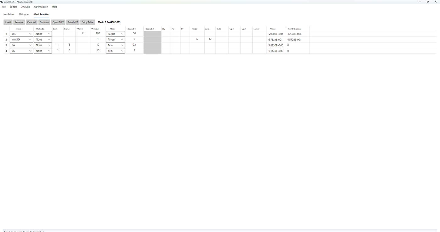
The Value column shows each row's live evaluation; the
Contribution column shows the row's residual squared (Error²).
On a well-aligned starting design the WAVEX Contribution dominates
— that's the operand the optimizer is actually working on. The
boundary rows contribute zero whenever the design is in-bounds.
Plus, in the Variable Editor, set Constraint = Min/Max on every
thickness variable (Min ≈ 1 mm for glass, Min ≈ 0.1 mm for air,
sensible Max values).
Four merit-function rows + bounded variables + a deliberate weight
hierarchy — that's the minimum for a well-protected optimization.
Add MAG, DITHETA, distortion bounds, etc. as your design's
specs require, and weight them in line with how strict the spec is.
Running the optimizer
Optimization → Local Optimization. The dialog opens with sensible defaults — Max Iterations 6000, Broyden Update on, Init Damp 1e-3 (Levenberg-Marquardt starting damping; see the optimization reference for when to override).
- Press Start. The dialog populates a per-variable table showing Start Value, Current Value, and Delta for every variable, and the merit value updates live in the header strip.
- Stop cancels mid-run; OK — Accept Results keeps the current state; Cancel — Revert restores the pre-run design.
On the Cooke-triplet starter — already a sensible triplet — the run converges almost instantly and improves the merit only modestly, from 0.0794 to 0.0757 (133 iterations, about 0.3 s on the native analytic engine). The header strip reports which engine actually ran (here Native Analytic):
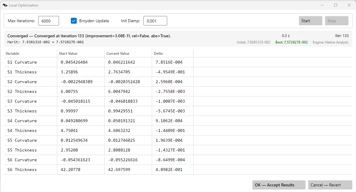
That few-percent gain is the defining trait of local optimization: it polishes the design you hand it — it does not transform it. Levenberg-Marquardt walks downhill to the nearest minimum of the merit surface and stops. Our starting triplet already sits close to a good local minimum, so "downhill" is a short walk.
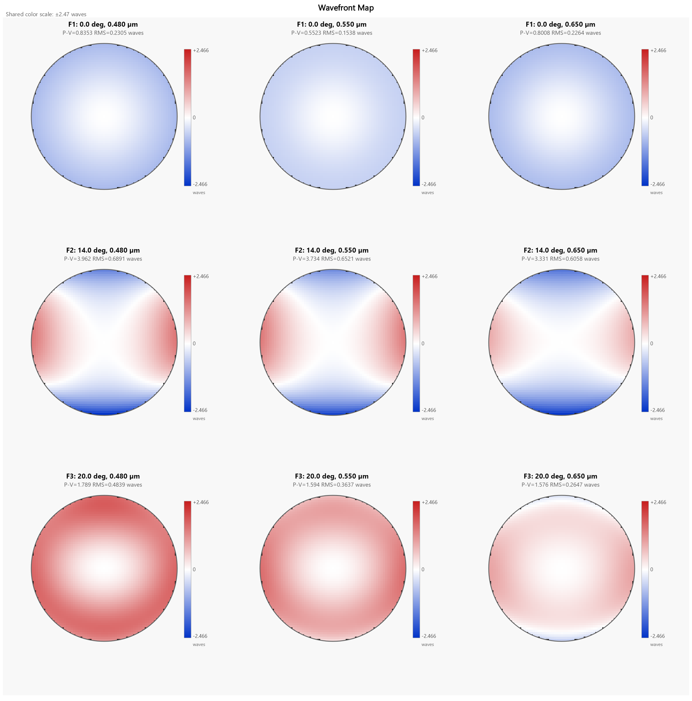
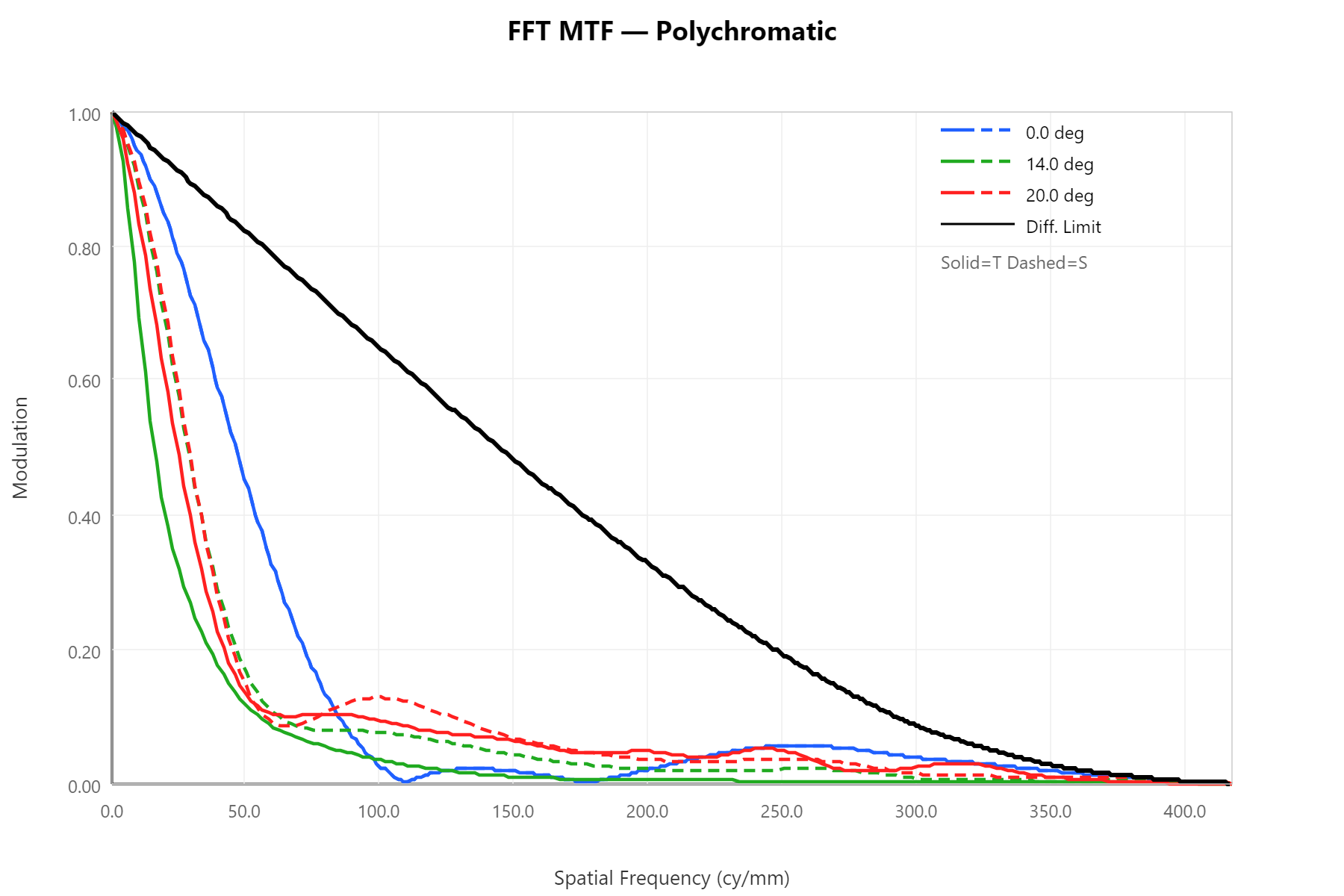
The before/after analyses make the point. The wavefront map and the polychromatic FFT MTF change only slightly — a small on-axis tidy-up, with the 14° and 20° fields essentially where they started (their oblique aberrations are baked into this glass/shape combination and a local polish can't reach them):
| Before (start, 0.0794) | After local opt (0.0757) | |
|---|---|---|
| Wavefront | 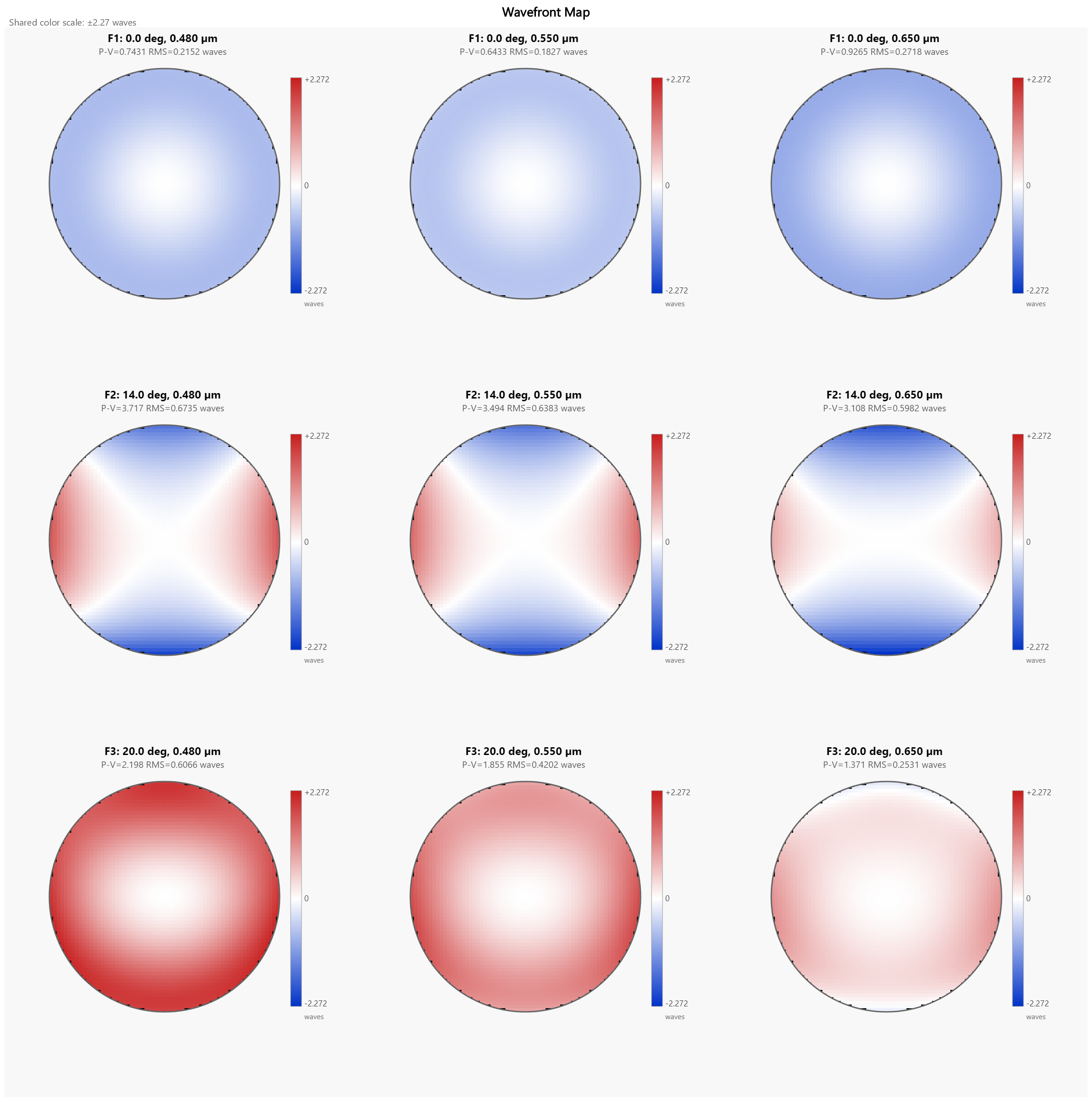 |
 |
| FFT MTF | 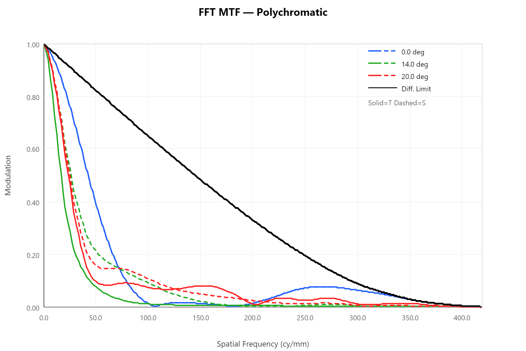 |
 |
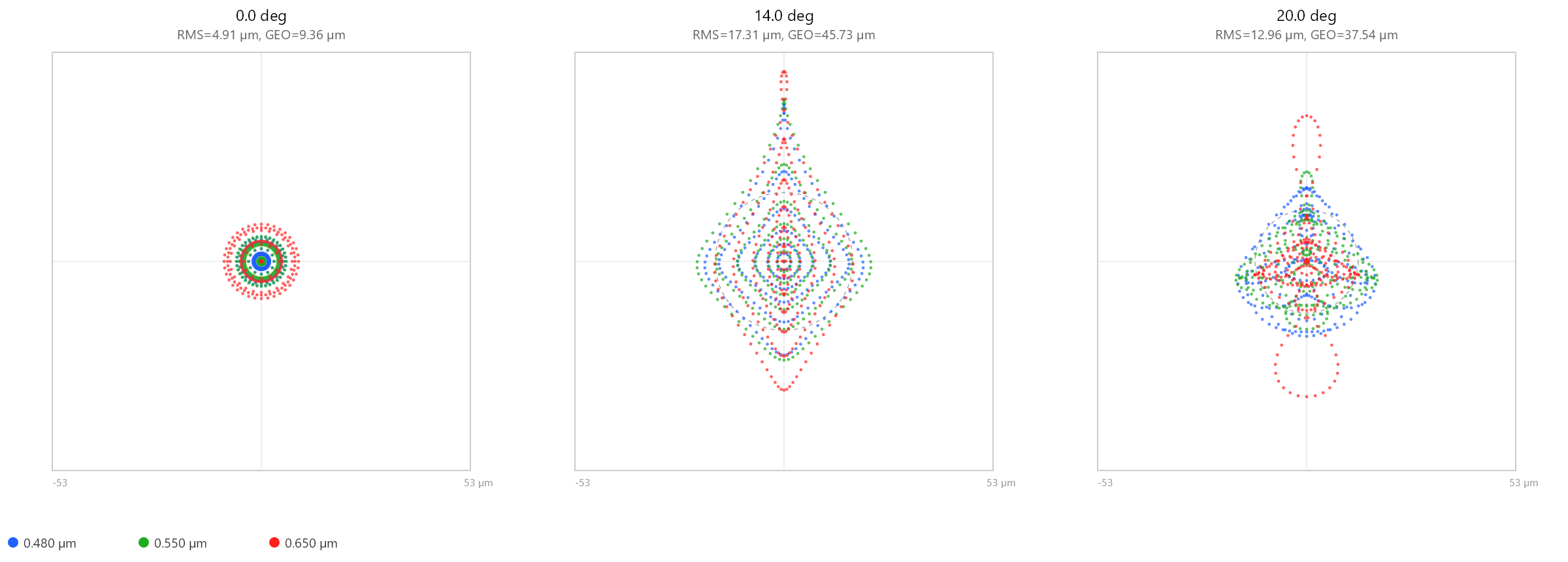
The geometric spot diagram barely moves at all — spot size here is dominated by the same off-axis aberrations that limit the off-axis MTF, so a local polish leaves it nearly untouched:
| Before (start) | After local opt |
|---|---|
 |
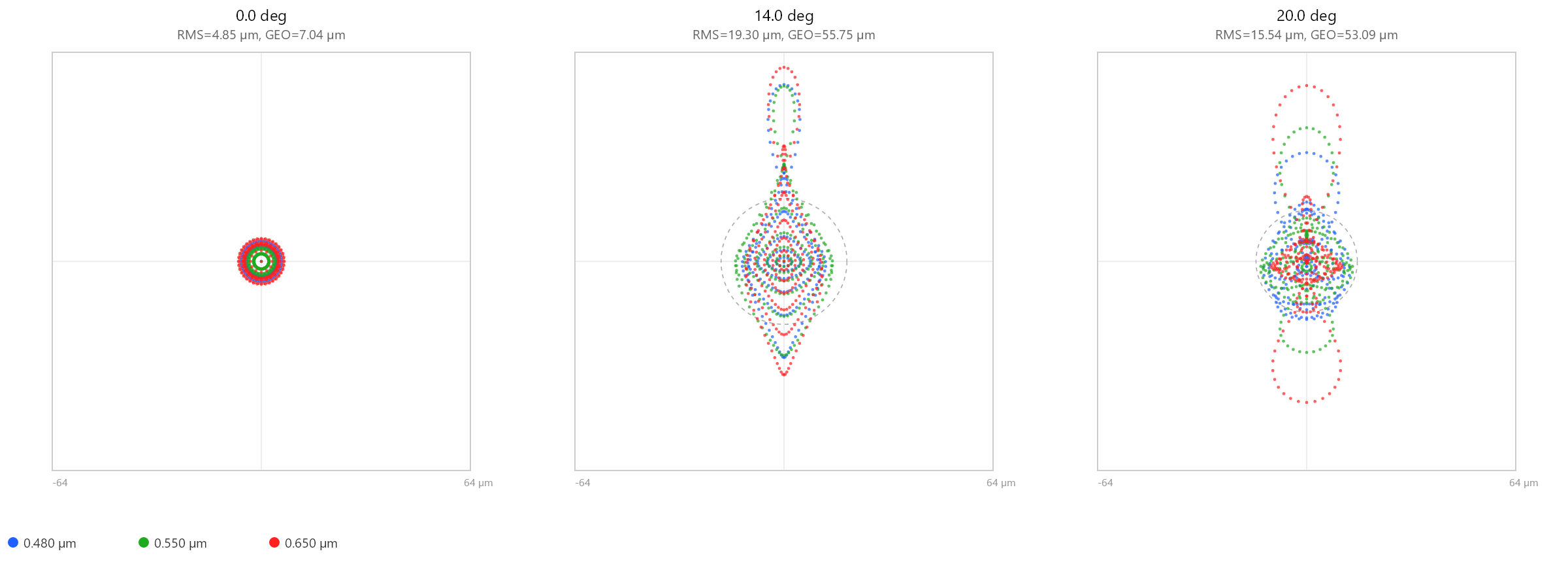 |
This is the moment to reach for a global method. To escape the starting basin — and to let the optimizer re-choose the glasses — see Multistart and Basin Hopping in the Optimization page. On this exact triplet they take the merit from 0.0794 all the way down to 0.0190, roughly a 4× improvement over this local polish, and in one demonstration they rebuild the whole lens starting from nothing but a stack of flat glass plates.
System Aperture & Object-Space Telecentric
The System Editor (System → System Editor) sets how the aperture is specified. Pick the Aperture Type and enter its Aperture Value:
| Aperture Type | Value means | Notes |
|---|---|---|
| EPD | Entrance-pupil diameter (lens units) | The classic default. |
| FNumber | Image-space F-number (EFL / EPD) | |
| Object Space NA | Object-space numerical aperture, NA = n₀·sin u (n₀ = the object medium's index = Surface 0's material) |
Finite-conjugate + Object Height fields only (see below). |
Object Space NA sizes the pupil from the marginal-ray cone leaving the object, which is the natural specification for finite-conjugate work (microscope objectives, relays, machine-vision lenses). It is valid only when the object is at a finite distance (Surface 0 has a finite thickness) and the Field Type is Object Height. If the system is infinite-conjugate or uses Object Angle fields, the System Editor shows a red warning and analyses / optimization return an error until you fix it.
Telecentric Object Space is a checkbox directly under the Afocal checkbox. When enabled, the entrance pupil is placed at infinity, so the chief ray is parallel to the optical axis in object space (the aperture stop appears at the front focal plane) — the standard condition for metrology and measurement optics, where magnification must not vary with object defocus. It is enabled only when the aperture is Object Space NA and Ray Aiming is Off; turning ray aiming on clears it. In the 2D layout you'll see each field's chief ray run parallel to the axis before the first surface.
Both settings are saved in .lhlt and round-trip through ZEMAX .zmx
(OBNA aperture; the object-space telecentric flag rides on the FTYP line).
File Types
| Extension | Meaning |
|---|---|
.lhlt |
LensHH-LT native format. Save/load from File → Save/Open. |
.zmx |
ZEMAX prescription. Import via File → Import ZMX. Only standard and even-asphere surfaces are honored. Object Space NA (OBNA) and object-space telecentric are honored. |
.agf |
Glass catalog. Loaded from <install>\catalogs\Glass\ on startup. |
Keyboard Shortcuts
| Shortcut | Action |
|---|---|
Ctrl+S |
Save |
Ctrl+O |
Open |
F5 |
Refresh all open analysis windows |
Esc |
Close the focused analysis window |
Analyses Reference
Each analysis opens its own tab from the Analysis menu (or its respective toolbar icon). Tabs update live when you change the system; pressing F5 in the main window forces a refresh of all open tabs.
The screenshots throughout this chapter come from the Cooke triplet
sample (samples/CookeTriplet.lhlt after a Local Optimizer pass) —
EFL 50 mm, F/5, three fields (0°, 14°, 20°), three wavelengths
(0.48 / 0.55 primary / 0.65 µm). Reusing one design across every
section lets you cross-reference what each analysis is showing you
about the same lens.
Common controls present on every tab:
- Wavelength — drop-down. Polychromatic aggregates across all system wavelengths weighted by their wavelength weights; individual entries show one wavelength.
- Field — which field points to show. Default is all fields.
- Compute — re-runs the analysis. Most tabs auto-compute on open and on system change; this button forces a recompute.
- Export Text… — saves the underlying numerical data as a TSV text file (the same one consumed by the validation suite).
- Export Image — saves the rendered plot as PNG.
- Show Table — pops up a tabular view of the data behind the curves.
- Close Tab — removes the tab. The next time you open the analysis from the menu it'll re-create the tab.
Spot Diagram
Analysis → Spot Diagram
Ray scatter on the image plane, one sub-plot per field, points colored per wavelength. In afocal mode the units switch to arcmin automatically.
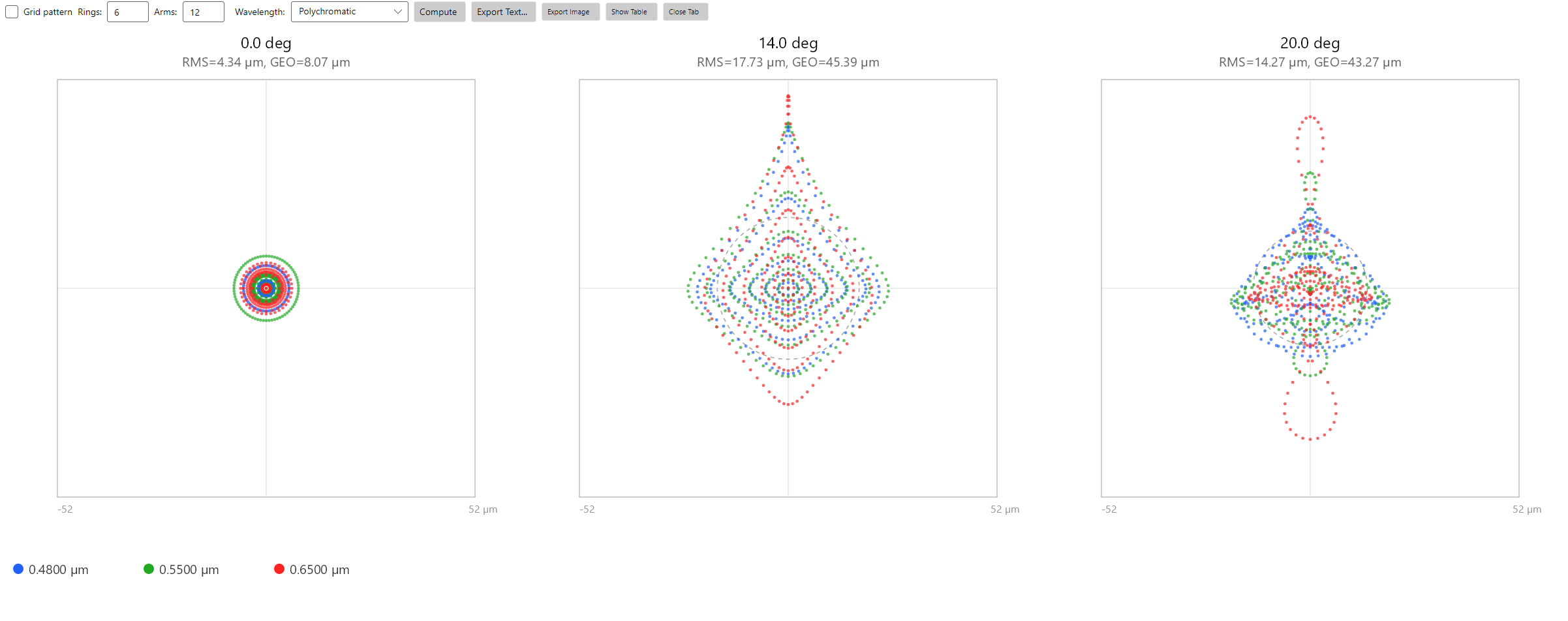
Reading the plot: above each sub-plot, RMS is the RMS spot radius about the centroid and GEO is the rim radius (worst-case ray). In the Cooke triplet above:
| Field | RMS | GEO |
|---|---|---|
| 0.0° | 3.76 µm | 8.07 µm |
| 14.0° | 15.41 µm | 46.05 µm |
| 20.0° | 12.53 µm | 43.42 µm |
The crosshair marks the chief ray; the star marks the centroid. The on-axis spot is dominated by spherochromatism (the 0.48 µm blue ring sits outside the others because secondary spherical aberration is wavelength-dependent). Off-axis the spots become diamond/heart shaped — characteristic coma + astigmatism mix you'd expect from a Cooke triplet at moderate field.
| Input | Meaning |
|---|---|
| Pattern | Hexapolar (Forbes-style ring × arm sampling) or Rectangular grid. |
| Rings / Arms | Hexapolar density. Default 6 × 12 = 72 rays per field per wavelength — matches the standard WAVEX / SPOT operand sampling. |
| Grid Size | Rectangular grid edge count. |
| Wavelength | One wavelength or all (polychromatic). |
With Polychromatic selected, RMS is the polychromatic
weighted RMS — the same value the SPOTM merit operand reports.
Transverse Ray Fan
Analysis → Ray Fan
Δx and Δy at the image plane for rays traced along the
meridional (Py) and sagittal (Px) pupil axes, plotted against
normalized pupil coordinate. One sub-plot per field, curves colored
per wavelength.
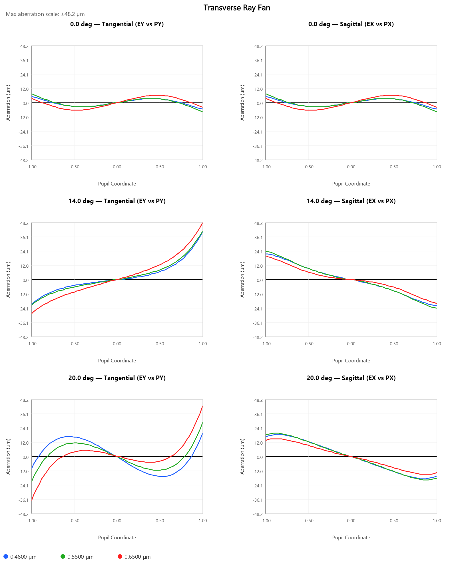
Read it for the same aberration signatures any transverse-ray-fan plot exposes:
- Slope at origin → defocus.
- Symmetric S-bow → spherical aberration.
- Asymmetric about origin in the meridional plot → coma.
- Difference between tangential and sagittal curves → astigmatism.
- Color separation → axial color (on-axis) or lateral color (off-axis).
Top row (0°): tiny, sub-µm aberrations — the Cooke triplet is essentially diffraction-limited on-axis. Middle row (14°): the tangential curve develops the asymmetric S-shape of coma; sagittal shows the symmetric astigmatism cup. Bottom row (20°): the same features grow, and the inter-wavelength color separation becomes visible (lateral color).
| Input | Meaning |
|---|---|
| Number of points | Samples per axis, default 20. |
| Wavelength | One wavelength or all. |
| Scale | Auto-scale both axes per field, or fix a common Y-range across all fields. |
OPD Fan
Analysis → OPD Fan
Optical path difference in waves, plotted against normalized pupil
coordinate along the meridional (Py) and sagittal (Px) axes.
Piston and tilt are removed — the same convention used by the
WAVEX merit operand.
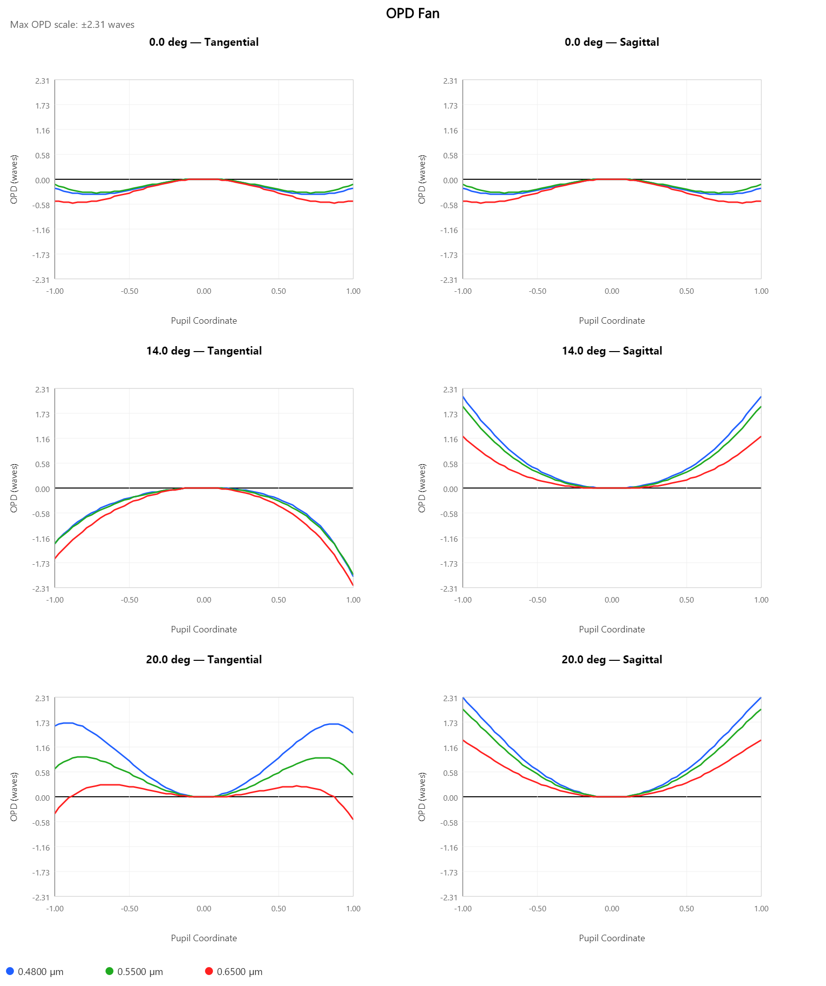
OPD sign convention: positive OPD = the test ray arrives ahead of the reference wavefront. The reference is the chief ray at the evaluation wavelength, corrected to the exit pupil for focal systems; for afocal systems the reference is a tilted plane wave.
Reading the plot is similar to the transverse-ray fan, but the shapes are integrals of the ray-fan curves (an antiderivative relationship): a parabolic OPD = defocus, a quartic OPD = spherical aberration, an asymmetric cubic = coma, etc.
In the Cooke triplet above the on-axis OPD stays well within ±0.5 waves across the band — diffraction-limited Marechal regime. The 14° tangential reaches –2 waves at the pupil edge (defocus + spherical residual), while 14° sagittal shows the ~+2-wave cup of astigmatism. The 20° tangential displays the M-shape characteristic of higher-order spherical mixed with field curvature; the inter-wavelength offset there is also the largest sign of chromatic content at the pupil edge.
The same OPD data feeds the wavefront map and the FFT PSF / FFT MTF analyses — anything that's a problem in the OPD fan will be a problem in those.
Pupil Aberration Fan
Analysis → Pupil Aberration Fan
Plots the pupil aberration — the difference between the real and paraxial pupil-position predictions for rays launched at each pupil coordinate. Useful for diagnosing systems where ray aiming matters (the chief ray doesn't actually pass through the real stop center even though we launched it through the paraxial pupil center).
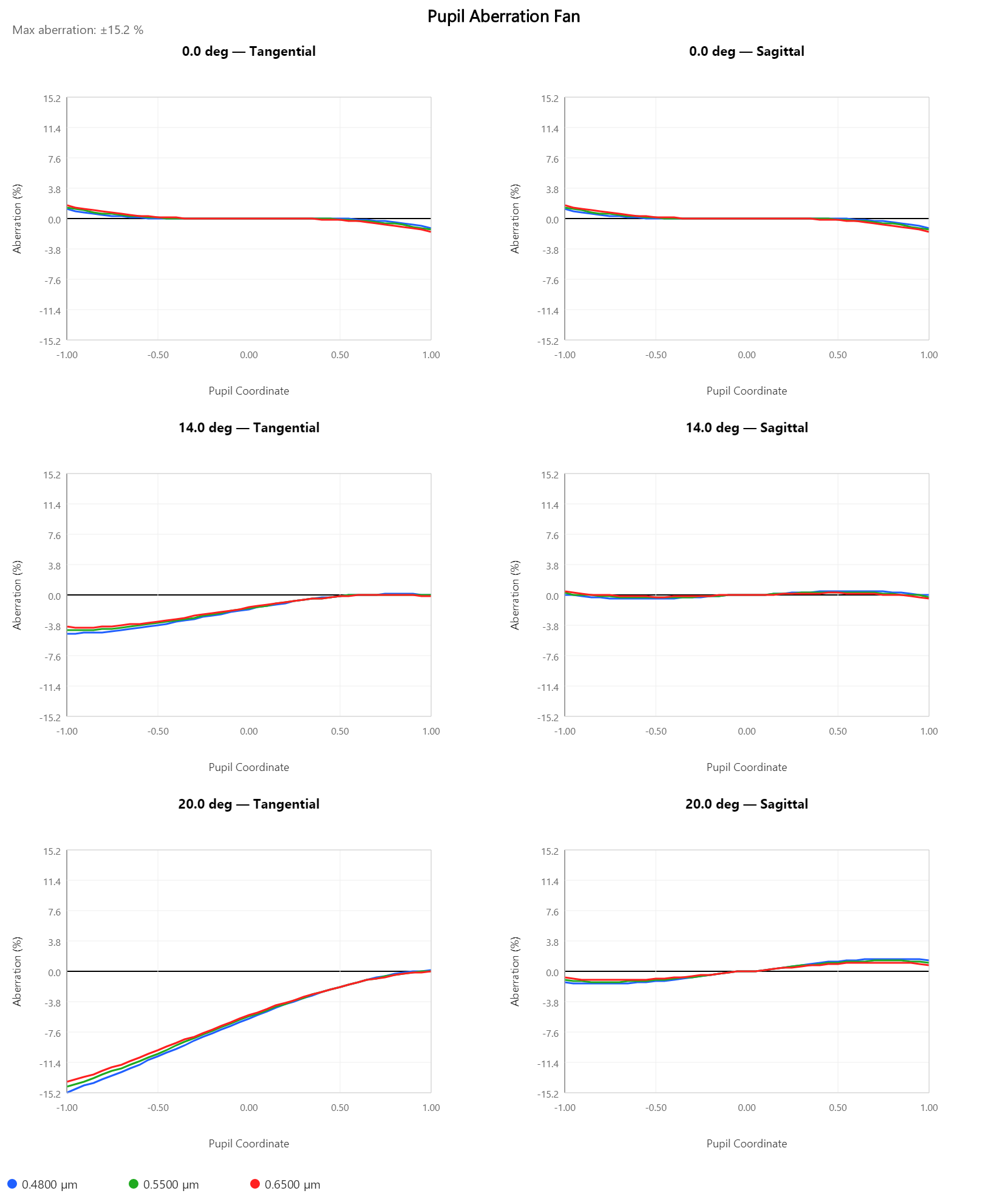
The Y-axis is "% of pupil radius the ray missed by." On-axis (0°) the pupil aberration is below 1 % — paraxial and real pupil positions agree closely. At 14°, tangential pupil aberration grows to ~4 % at the edge of the pupil; at 20° tangential it reaches ~–15 % — meaning rays launched at full pupil edge actually arrive –15 % short of where paraxial says they should.
When this number is large (> 5 % at the field of interest), turning Ray Aiming = Real in the System Editor materially changes the merit-function values and the FFT MTF — Multistart and Basin Hopping will converge to slightly different optima with vs without ray aiming for such systems.
For typical lenses with modest field and well-placed stop, pupil aberration is small and ray aiming makes negligible difference.
Wavefront Map
Analysis → Wavefront Map
Color map of OPD across the pupil (the 2D version of the OPD fan).
Tilt and piston are removed — same convention as WAVEX. Contour
lines optional.
| Input | Meaning |
|---|---|
| Pupil Samples | Grid resolution. Larger = slower but smoother. Default 64. |
| Wavelength | One or polychromatic. |
| Field | One field at a time. |
| Color scale | Auto-fit per field, or fix a global waves range. |
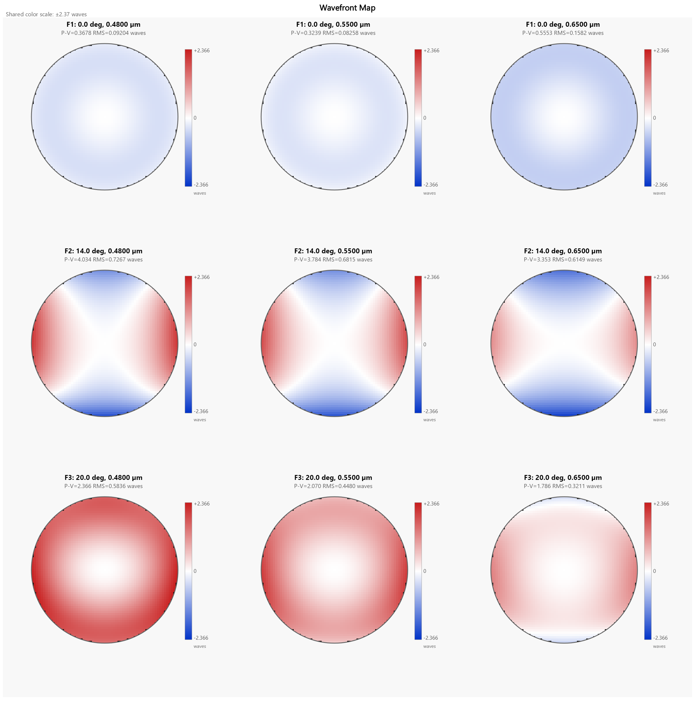
Above each sub-plot: peak-to-valley (P-V) OPD and RMS, both in waves at the evaluation wavelength. The wavefront map is the clearest single picture of an aberrated bundle's pupil structure — spherical aberration appears as concentric rings, coma as a tilted asymmetry, astigmatism as a saddle, and so on.
The same OPD that feeds the FFT PSF and FFT MTF is the wavefront map you see here.
FFT PSF
Analysis → FFT PSF
Diffraction-based point-spread function at one field, computed by
FFT of the pupil amplitude (apodized by transmission) and the
complex wavefront exp(i 2π OPD).
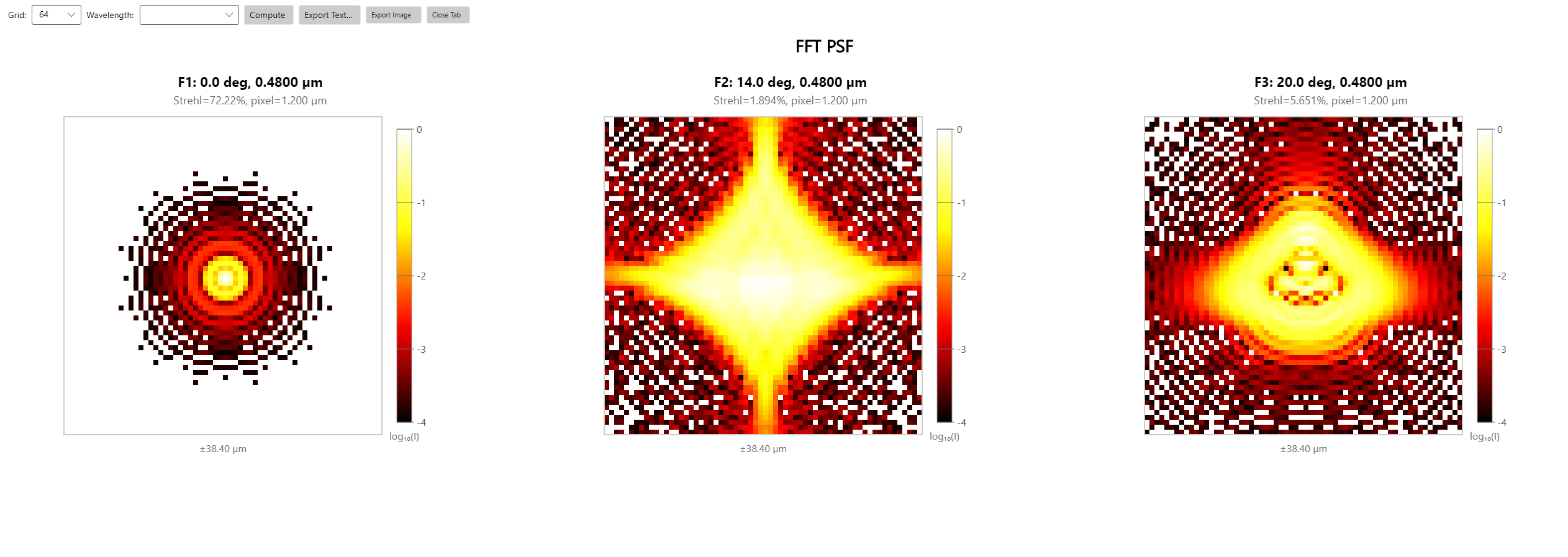
| Input | Meaning |
|---|---|
| Pupil Samples | FFT grid edge size. Power of 2; typical 256 or 512. |
| Display Size | Image-plane extent shown (µm). |
| Field | One at a time. |
| Wavelength | Individual wavelength or polychromatic (incoherent sum of per-wavelength PSFs, weight-averaged). |
Reported metrics (above the image): peak intensity normalized to the diffraction-limited peak (= Strehl ratio) and peak position relative to the chief ray.
Use the FFT PSF to inspect the actual image of a point source — useful for predicting how a star or pinhole will look on the sensor. For broadband systems, the polychromatic PSF is the right choice; the monochromatic PSF tends to show diffraction rings that average out across a real source.
FFT MTF vs Frequency
Analysis → FFT MTF
Diffraction modulation transfer function vs spatial frequency for
each field, tangential (solid) and sagittal (dashed). Computed by
FFT of the geometric-pupil PSF; accuracy is set by the Pupil
Samples grid (truncation error falls roughly as 1/N² for an
N × N grid).
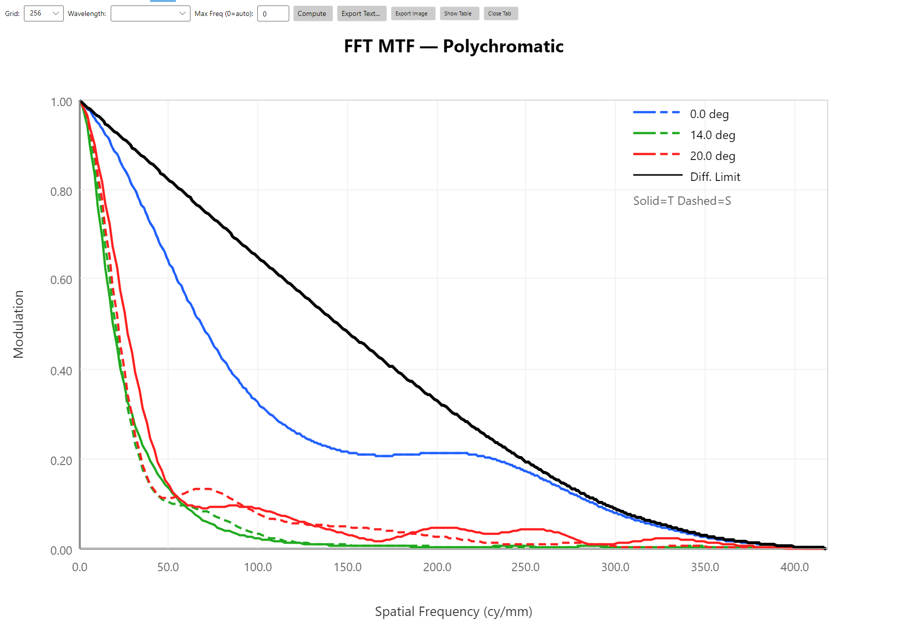
| Input | Meaning |
|---|---|
| Max Frequency | 0 = auto (use the diffraction cutoff). Otherwise truncate at this value (cycles/mm for focal, cycles/mrad for afocal). |
| Pupil Samples | FFT grid. Typical 64 or 128. |
| Wavelength | Individual wavelength or polychromatic. |
The displayed cutoff is the canonical projection ρ_T × f_axial
for tangential and ρ_S × f_axial for sagittal, where
ρ = cos(θ_chief_image) (Macdonald 1971, eq 4.4 evaluated at the
axially-symmetric paraxial limit). On-axis ρ = 1 and the cutoff
is the full diffraction limit 1 / (λ × F/#). Off-axis the cutoff
is reduced by the chief-ray cosine projection.
Afocal systems automatically switch to cy/mrad, matching the spot-diagram unit convention.
FFT MTF vs Field
Analysis → FFT MTF vs Field
Tangential and sagittal MTF at one (or several) fixed spatial frequencies, plotted against field. Useful for flatness-of-field inspection — does the corner of the image hold MTF, or does it collapse?
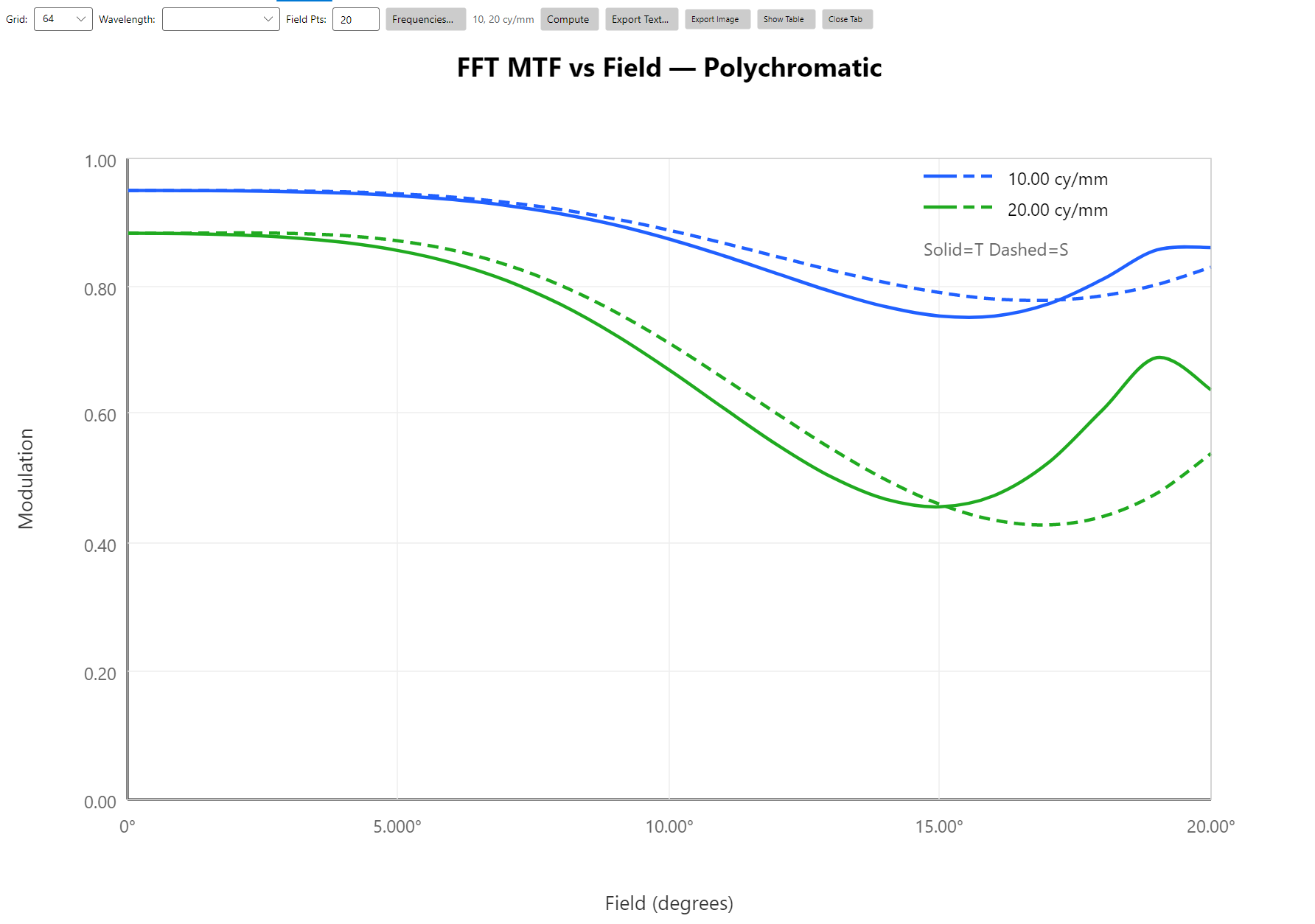
| Input | Meaning |
|---|---|
| Frequencies | One or several spatial frequencies (cy/mm) to evaluate. Default 10 and 20 cy/mm. |
| Pupil Samples | As above. |
| Field Pts | Number of field samples between 0 and max field. |
FFT MTF Through Focus
Analysis → FFT MTF Through Focus
MTF at a single spatial frequency and field, plotted against an image-plane offset. The peak of each curve marks best focus for that field at that frequency; the spread between fields shows field curvature converted into modulation.
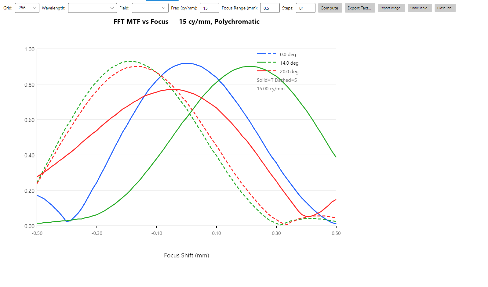
| Input | Meaning |
|---|---|
| Frequency | Spatial frequency to evaluate (cy/mm). |
| Δz range | Image-plane offset sweep (mm). |
| Steps | Number of focus positions. |
Geometric MTF
Analysis → Geometric MTF
Geometric MTF computed by Kidger's Gaussian-quadrature method as described in Michael J. Kidger, Fundamental Optical Design (SPIE Press, 2002). The pupil is sampled on a Gauss-Legendre ring × arm grid, real rays are traced to find the geometric spot, the spot intensity is Fourier-transformed to give the geometric OTF, and the result is multiplied by the diffraction-limited MTF for the appropriate field-dependent cutoff.
The diffraction-limit multiplication is intentional: pure geometric MTF can rise above the diffraction limit at moderate spatial frequencies in nearly diffraction-limited systems, which is non-physical. Multiplying by the DL gives a curve that's a better proxy for the actual modulation when both aberration and diffraction contribute. At low frequencies (geometric regime, aberrations dominate) the curve is essentially the geometric prediction; near and past the DL cutoff the multiplication forces it toward zero.
Three variants share the same Kidger engine and parameters:
Geometric MTF vs Frequency
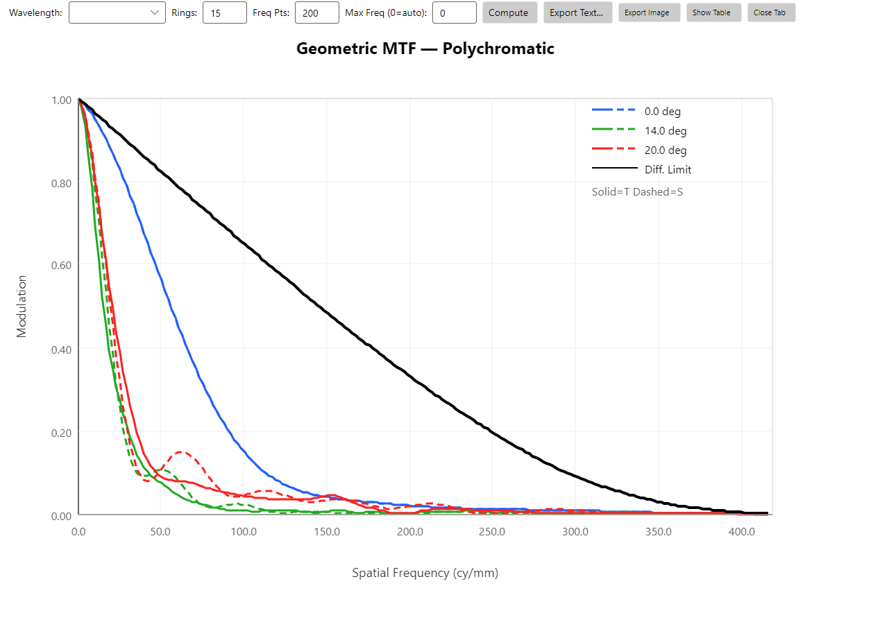
Curves: 0° (blue) tracks the diffraction limit out past 50 cy/mm and is close to diffraction-limited overall. 14° (green) and 20° (red) drop fast — aberrations dominate from below 30 cy/mm. The scalloped shape at higher frequencies is real OTF structure (zero crossings of the spot autocorrelation), not numerical noise.
Geometric MTF vs Field
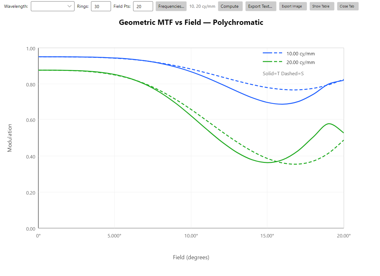
Holds the spatial frequency fixed (10 and 20 cy/mm in the screenshot) and sweeps the field from on-axis to maximum. Reading the 10 cy/mm trace: ~0.95 modulation through 5°, dropping to ~0.7 at 15°, and recovering somewhat at 19°-20° — the recovery near maximum field is a sign that the design's residual aberration reverses sign there.
Geometric MTF Through Focus
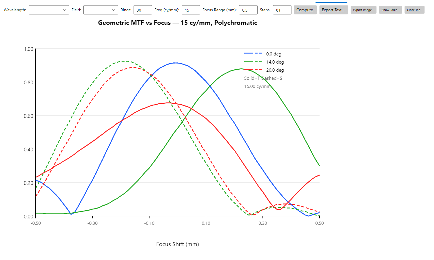
15 cy/mm modulation as a function of Δz. The 0° (blue) and 14° (green) tangential peaks are offset along the focus axis — that's the field curvature converted into MTF terms. The 20° (red) tangential is broader and lower, mostly because the 20° spot is also broader (see the Spot Diagram). Choose your image-plane position to maximize the worst-field MTF, not the on-axis MTF.
| Input (all variants) | Meaning |
|---|---|
| Rings | Gauss-Legendre quadrature rings on the pupil. Default 15 (vs-frequency) or 30 (vs-field / through-focus). |
| Field Pts | Field samples (vs-field, through-focus). |
| Frequency / Frequencies | cy/mm (or cy/mrad afocal). |
| Wavelength | One or polychromatic. |
Field Curvature
Analysis → Field Curvature & Distortion
Tangential (solid) and sagittal (dashed) best-focus position vs field, plotted as Focus Shift (mm) along the X-axis and field along the Y-axis (matches the standard convention).
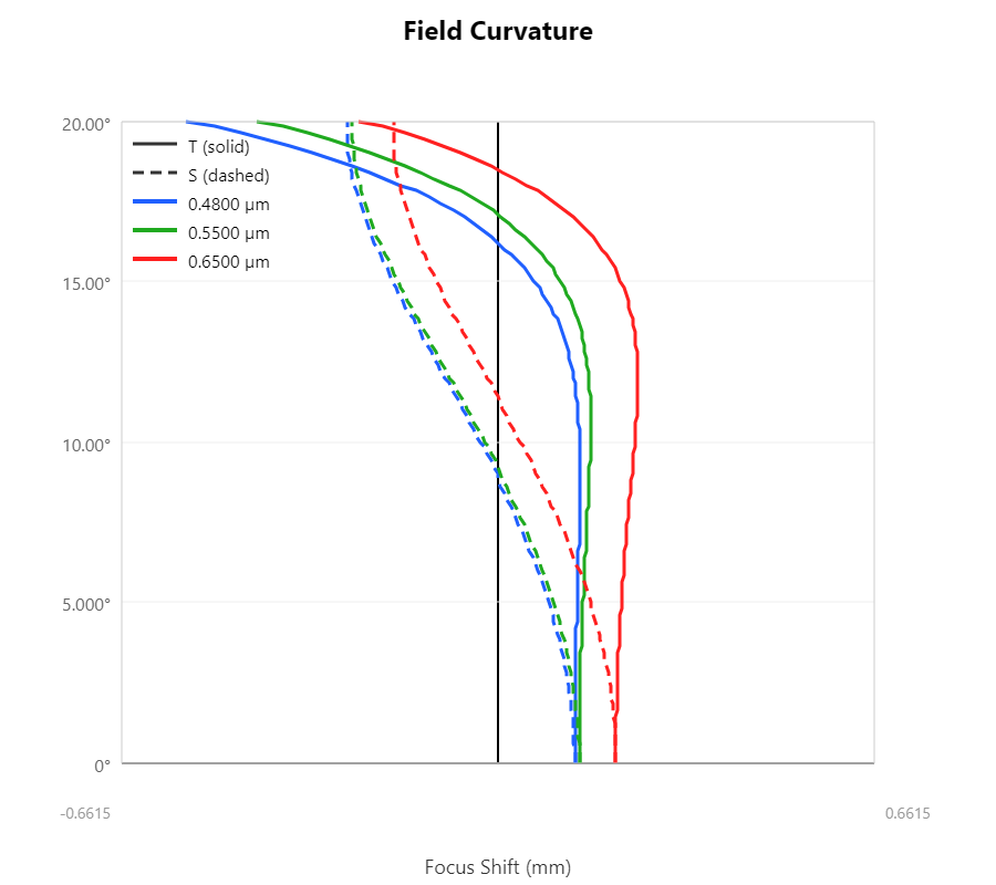
The intersection of the T and S curves at each field is the Petzval surface for that wavelength; the gap between T and S at a given field is the astigmatism. In the Cooke triplet:
- 0°-10° fields: T and S essentially overlap and stay within a few hundred microns of paraxial focus — the design is well-corrected in the inner field.
- 10°-20°: tangential and sagittal pull apart, with tangential bowing forward (smaller Z) and sagittal staying closer to flat. The maximum T-S separation at 20° is ~0.4 mm — the astigmatism budget at the field edge.
- Across wavelengths: the three curves are roughly parallel and shifted along Z — that's chromatic field curvature (longitudinal color × field curvature).
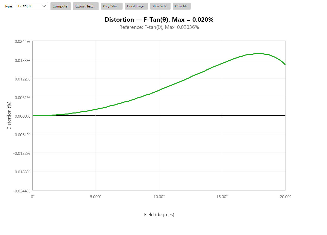
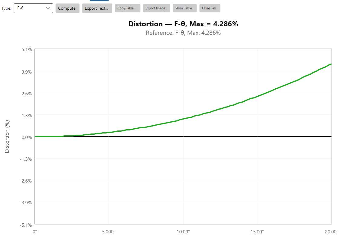
Distortion
Analysis → Field Curvature & Distortion, Type: F-Tan(θ) or F-θ
Percent distortion vs field. The reference focal length is computed
from the slope dY/d(tan θ) of the chief ray near zero field — a
finite-difference between two small angles that removes any
constant chief-ray pupil-aberration bias and gives the true
effective focal length the chief ray actually sees. Same approach
as the DITAN / DITHETA merit operands.
Two reference types are selectable:
- F-tan(θ): ideal
h = f × tan(θ). The standard rectilinear imaging convention. Cameras and most photographic lenses target this. - F-θ: ideal
h = f × θ. The scanner-lens convention, where a constant angular increment maps to a constant linear increment on the image — needed for laser scanners, document scanners, etc.
For the same Cooke triplet at the same fields, the two references tell different stories:
| F-Tan(θ) | F-θ |
|---|---|
 |
 |
F-Tan(θ): max 0.020 % at ~17° field. The Cooke triplet is a well-corrected rectilinear lens; F-tan(θ) distortion is naturally tiny.
F-θ: max 4.286 % at 20°. The same lens looks 200× worse against an F-θ reference, because the lens is not an F-θ lens — F-θ scanner lenses require a fundamentally different design with strong negative third-order distortion built in to compensate. This view is useful only if you actually need an F-θ output; for imaging applications the F-tan(θ) plot is what matters.
Relative Illumination
Analysis → Relative Illumination
Relative illumination as a function of normalized field:
RI(H) = (F/#_on-axis / F/#_field)²
Computed by tracing rays in 24 azimuthal directions (boundary search) to measure the actual transmitting cone at each field, comparing to the on-axis cone.
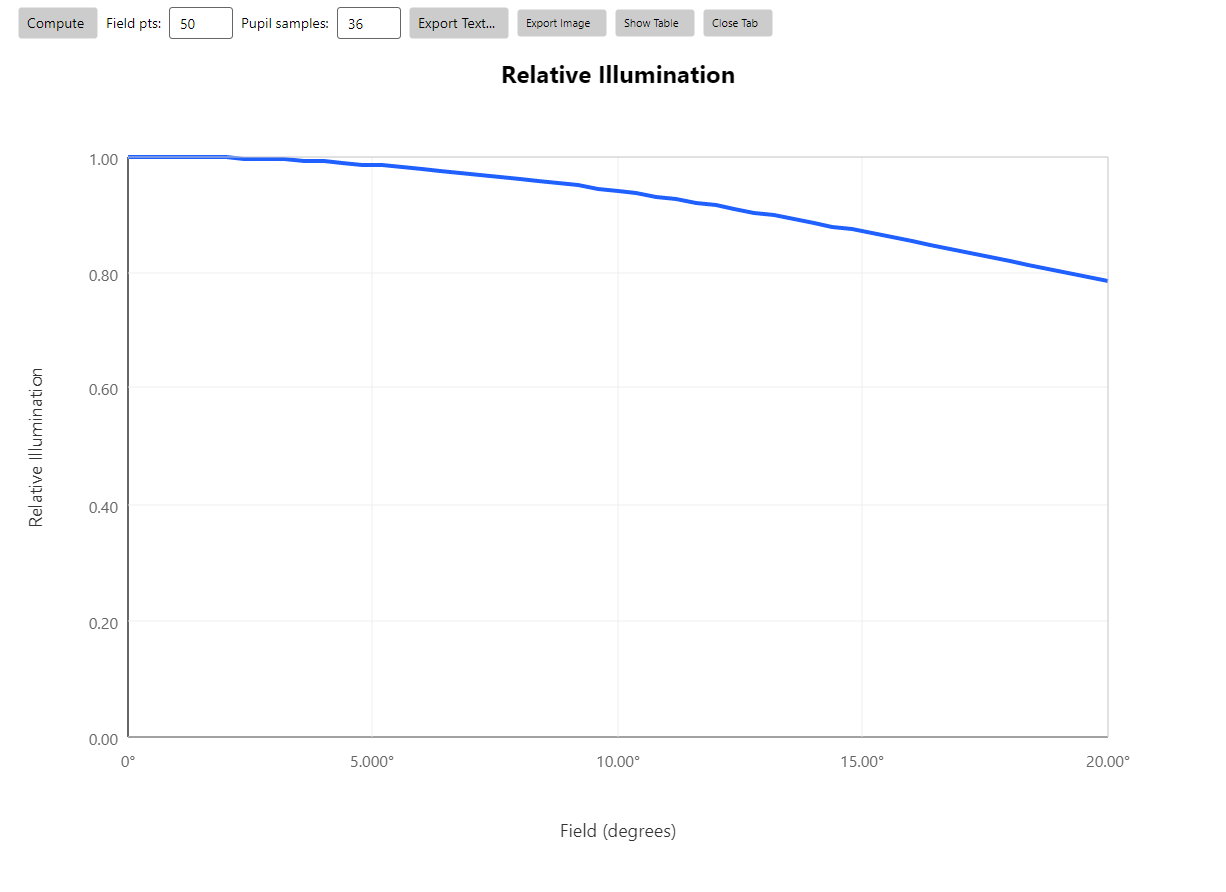
Reading: at 20° the Cooke triplet transmits ~79 % of the on-axis
illumination. Nearly all of that drop is the geometric cos⁴(θ)
effect (cos⁴(20°) ≈ 0.78); for a system with vignetting the curve
would drop substantially faster than cos⁴.
| Input | Meaning |
|---|---|
| Field pts | Field samples between 0 and max. Default 50. |
| Pupil samples | Boundary-search azimuth count. Default 36 — increase to 48 or 72 for systems with sharp vignetting boundaries. |
The same RI operand is available in the merit function — see
Merit Function Reference
— and uses the same boundary-search routine.
For wide-angle and retrofocus designs the curve can briefly exceed 1.0 (apparent concentration off-axis from pupil walking); that's not a bug.
Lateral Color
Analysis → Lateral Color
Chief-ray image-height difference at each non-primary wavelength
relative to the primary wavelength, plotted vs field. Output in µm
(focal mode) or arcmin (afocal mode). Matches the LCF merit
operand.
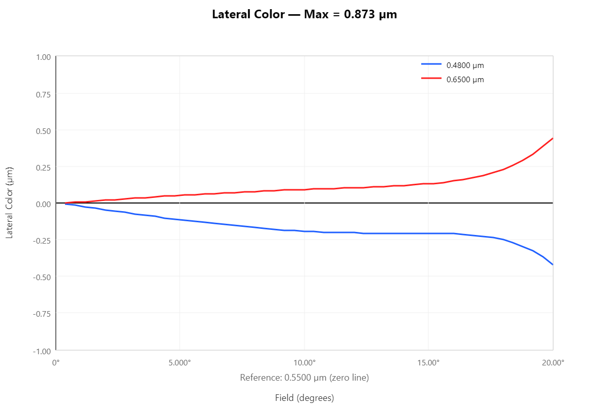
The reference (zero line) is the primary wavelength — the curves show how far the other wavelengths' chief-ray heights deviate from it. In the Cooke triplet the 0.48 µm (blue) and 0.65 µm (red) spread is ≤0.5 µm out to about 16°, then widens to ~0.87 µm at the 20° field edge. The spread between extreme wavelengths at any given field is the lateral chromatic aberration at that field.
The reported Max value at the top is the maximum across all
fields and all non-primary wavelengths — the same number LCF
returns when used at full field.
Chromatic Focal Shift
Analysis → Chromatic Focal Shift
Paraxial best-focus offset vs wavelength, plotted as a curve. The offset is image-plane Z displacement (µm) for focal systems and a diopter shift for afocal systems.
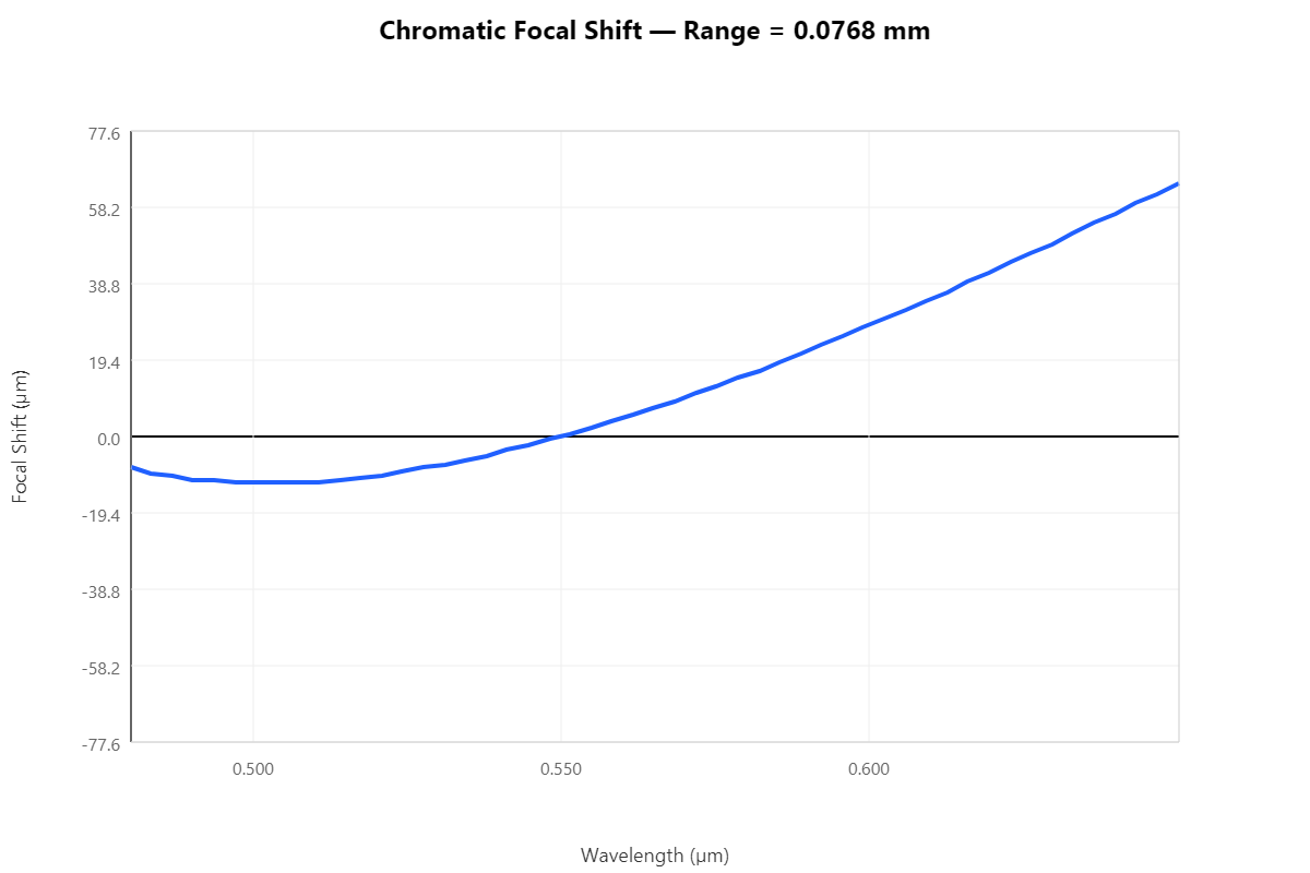
The zero line is the primary wavelength's focus position. Reading the Cooke triplet curve: F-line (0.48 µm) sits at ~–8 µm relative to d-line, blue → green crosses zero, and C-line (0.65 µm) is at +62 µm — so the long-wavelength focal length is significantly longer than the short-wavelength focal length. This is secondary spectrum — the residual color a thin two-glass achromat can't fully correct. Three-glass apochromats reduce this to a few µm; a Cooke triplet only partially corrects it.
The title shows Range = peak-to-peak focal shift across the swept wavelength interval.
| Input | Meaning |
|---|---|
| Wavelength grid | Number of sampled wavelengths between the system's min and max. Default 50. |
Longitudinal Aberration
Analysis → Longitudinal Aberration
For each system wavelength, sweeps the entrance pupil from the axis out to the marginal zone and plots the focus shift — the axial distance from the image plane to where that zone's marginal ray crosses the optical axis. One curve per wavelength.
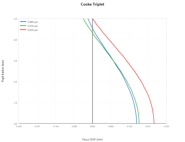
Two distinct things are visible on a single plot:
- Spherical aberration — the curvature of any single-wavelength trace. A vertical line would mean every pupil zone focuses at the same axial position; the deviation from vertical is the longitudinal spherical aberration. Reading the Cooke triplet's green (0.550 µm) curve: paraxial focus sits at about +0.20 mm relative to the image plane, marginal focus around −0.05 mm — a ~0.25 mm undercorrected SA characteristic of an f/5 triplet.
- Axial chromatic aberration — the horizontal spread between curves at any fixed pupil zone. At the paraxial (zone 0) point: blue is at +0.19 mm, green at +0.20 mm, red at +0.28 mm — the red focus is significantly further from the image plane than the blue. This is the same axial color reported by the Chromatic Focal Shift analysis, viewed in cross-section.
The reference (the vertical line at 0) is the system's paraxial focus at the primary wavelength. For infinite-conjugate systems this equals the paraxial BFL; for finite-conjugate systems it is the on-axis object's paraxial image distance (which moves with the object distance — the analysis tracks this automatically).
| Input | Meaning |
|---|---|
| Number of zones | Pupil samples between axis and full aperture. Default 32. |
Seidel Coefficients
Analysis → Seidel
Surface-by-surface third-order aberration coefficients with system
totals. Bar chart with one column per surface plus a SUM column;
each column has seven bars for the seven coefficient categories.
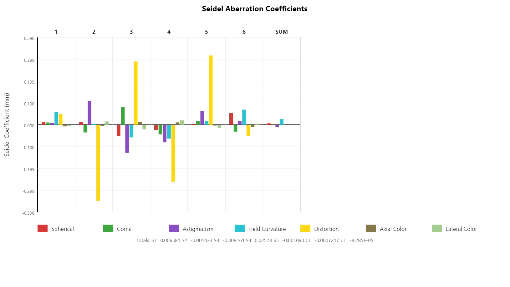
The seven categories:
| Symbol | Aberration |
|---|---|
| S1 | Spherical |
| S2 | Coma |
| S3 | Astigmatism |
| S4 | Petzval (field curvature) |
| S5 | Distortion |
| CL | Axial color |
| CT | Lateral color |
Bar height is the contribution of that surface to the system total
(in mm, except CL/CT which are in waves). The SUM column on the
right is the system total for each coefficient.
In the Cooke triplet screenshot, surfaces 2 and 3 contribute large
opposing distortion values (yellow bars at –0.32 and +0.29 mm) —
that's the classic positive-negative-positive cancellation a Cooke
triplet uses for field correction. The SUM distortion total (S5
in the legend) is much smaller than any single contribution
because of this cancellation.
The header shows the Totals: line with the seven sums. Glance at
this to see which coefficient is dominant; then look at the
per-surface bars to identify which surface is most responsible —
that's the surface to vary first when you optimize against that
coefficient.
| Input | Meaning |
|---|---|
| Wavelength | One wavelength at a time (defaults to primary). |
Values follow the standard third-order convention.
Zernike Coefficients
CLI / MCP / API only — no GUI page. Run via
lhlt analyze zernike(CLI), thelhlt_analyze_zernikeMCP tool, orLensHHSession.AnalyzeZernike(...)in the API. Tabular output is produced byZernikeTextExport.
Decomposes the wavefront at one (field, wavelength) into Zernike
polynomial coefficients. Two ordering conventions are available:
- Fringe (sometimes "University of Arizona"): 37 terms, ordered by ascending mode-set within each radial order. Standard output for many interferometric instruments.
- Standard (Noll): 36 terms ordered by
nthenm. Standard for atmospheric / telescope work.
| Input | Meaning |
|---|---|
| Number of terms | How many coefficients to fit. Default 37 (Fringe) / 36 (Standard). |
| Pupil Samples | Grid resolution for the fit. |
| Field / Wavelength | One of each. |
| Convention | Fringe or Standard. |
The piston (Z1) and tilt (Z2, Z3) terms are typically tiny — unaberrated tilt has been removed in the wavefront. The dominant Zernike modes for a well-corrected lens are usually defocus (Z4), spherical (Z9 / Z11 in Fringe), and the lower-order coma / astigmatism modes.
Use the Zernike table to identify which aberration is dominant in a residual wavefront — much faster than guessing from the shape alone.
Single Ray Trace
Analysis → Single Ray Trace
Trace one ray at a user-specified (field, wavelength, pupil) and
list its full state at every surface: position, direction cosines,
optical path length, accumulated waves, AOI (angle of incidence)
and AOE (angle of exitance).
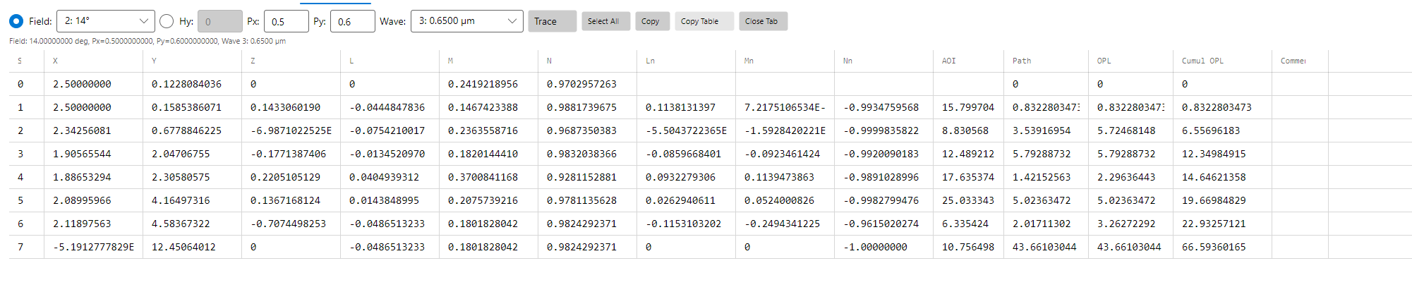
| Input | Meaning |
|---|---|
| Field index | 0-based index into the system's field list. |
| Wavelength index | 0-based index into the wavelength list. |
| Px / Py | Normalized pupil coordinate (–1 to +1). (0, 0) = chief ray; (0, 1) = upper marginal; (1, 0) = sagittal marginal. |
Use this when a higher-level analysis is giving a surprising
answer and you want to step through one ray manually. The same
ray-trace results are exposed in the merit function via the RX /
RY / AOID / etc. operands.
System Data
Analysis → System Data
Summary table of first-order properties and derived scalars:
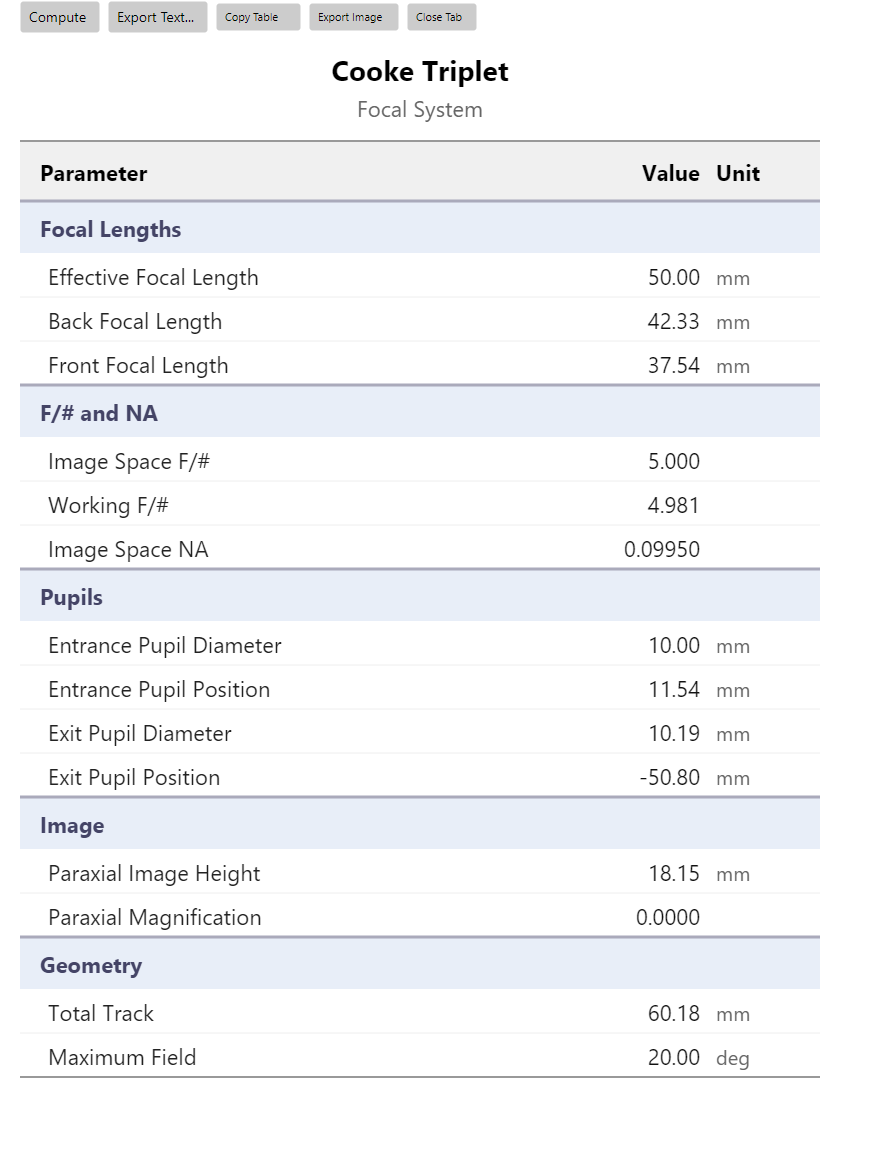
- EFL — paraxial effective focal length.
- F/# — system F-number (computed from EFL and entrance pupil diameter).
- BFL — back focal length (last surface to paraxial focus).
- Total track — first surface to image plane.
- Entrance / exit pupil — diameter and z-position.
- Numerical aperture — image-side NA.
- Field angles / heights — the user's field list.
- Image-side angles / heights — chief-ray image positions.
No inputs. Updates whenever the system changes.
Layout
Analysis → 2D Layout
2D profile view of the lens with surface outlines, glass shading, and rays from each field in each wavelength. Useful for sanity- checking that chief rays do reach the image plane and that the aperture stop is where you expect.
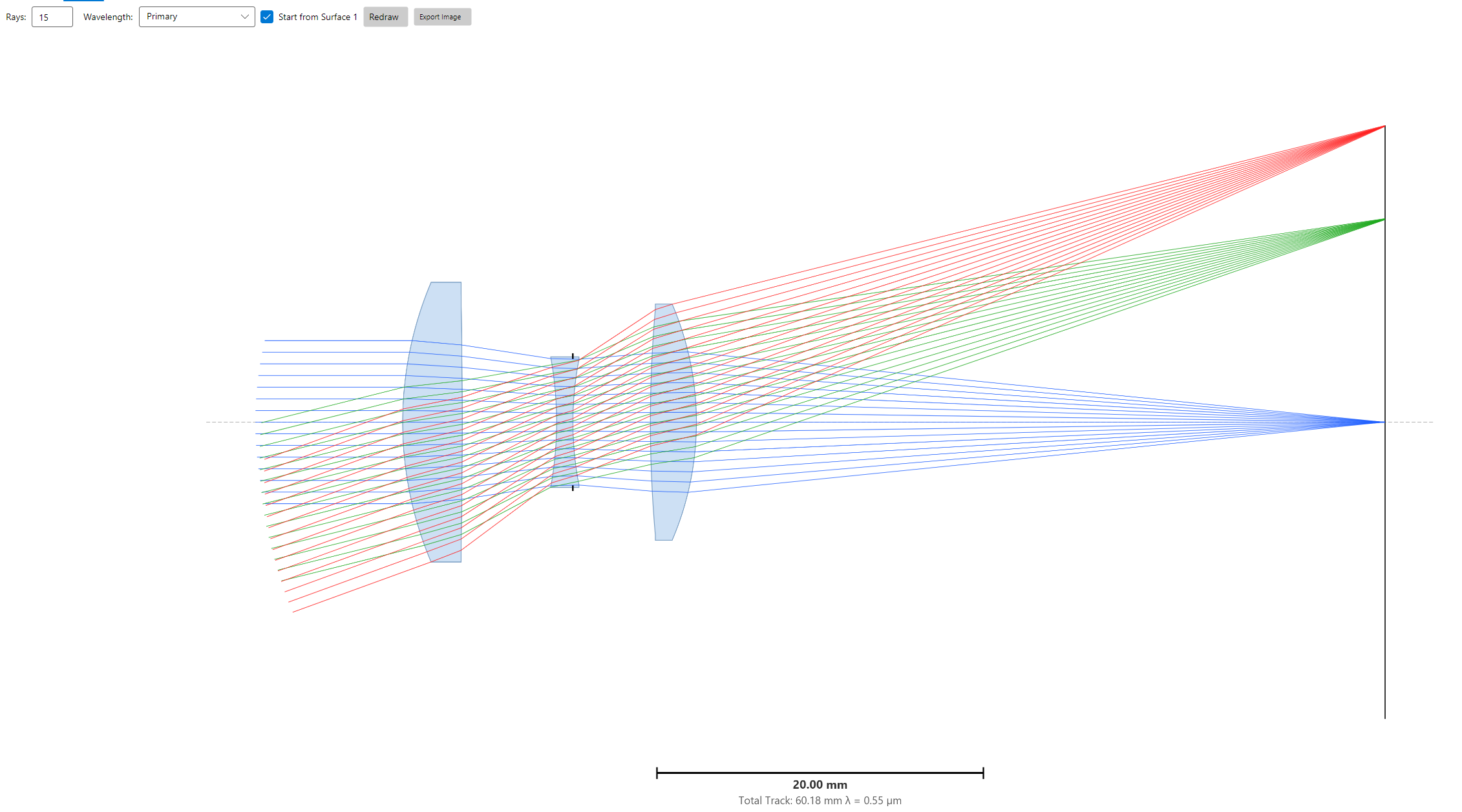
| Input | Meaning |
|---|---|
| Rays per field | Number of pupil rays drawn between the +py and –py marginals. |
| Wavelength filter | Draw one or all wavelengths. |
| Layout mode | Off (paraxial pupil aiming), Real (real-ray-aimed), or Robust (wide-angle iterative search). Match this to the system's RayAiming setting if you're cross-checking against the merit function. |
The 2D Layout is also available as its own always-on tab from the sidebar — use that for live editing while watching ray paths update; use the dedicated Analysis-menu version when you want a captured image for a report.
Performance and Accuracy Tips
- Cache-friendliness. Opening many analysis tabs at once is fine; each one caches its own ray traces. But an optimization run re-evaluates after every iteration — close analysis tabs during long optimizations if your machine feels sluggish.
- Pupil samples are power-of-2. FFT-based analyses pad internally to the next power of 2. Picking 64 / 128 / 256 directly avoids the wasted pad cost.
- Afocal systems. All angular outputs (spot, lateral color, chromatic focal shift in diopters, MTF in cycles/mrad) switch automatically. No manual unit change needed.
- Obscurations. Central obscurations declared in the system aperture are honored — pupil sampling skips the obscured inner disk and Seidel / Zernike fits use the annular weight.
- Field Y vs field height. When
FieldType = ObjectAngle, field values are degrees; whenFieldType = ObjectHeight, they are millimeters. The plots show the correct unit on the X-axis in both cases.
Merit Function Reference
The merit function is a list of operands. Each operand produces one value; the optimizer drives the weighted sum of squared residuals to zero. A residual is the operand's value minus its target (in Target mode), or the distance outside its Min/Max bounds (in Boundary mode).
Operand Row — Common Columns
Every operand has these columns in the Merit Function Editor:
| Column | Meaning |
|---|---|
| Type | The operand type (e.g. SPOT, EFL, CTG). Determines what the operand computes. |
| Mode | Target (drive toward a value) or Min/Max (penalize if outside a bound). |
| Target / Min / Max | The reference value for the chosen mode. |
| Weight | Multiplier on the residual. 0 disables the row. |
| OpCode | Optional post-processing: Abs, Sqrt, Sin, Cos, Tan, Asin, Acos, Atn. Default None. |
| Value | Read-only — the last-computed value. |
The remaining columns depend on the operand type (see each category below). Columns irrelevant to the selected type are greyed out.
Spot Operands
Diffraction-quality merit — RMS transverse ray aberration over pupil quadrature.
| Type | Reference | Sampling | Notes |
|---|---|---|---|
SPOT |
Chief ray | Forbes Gauss-Legendre quadrature (Rings × Arms) |
Tracks TRAD/TRAE per pupil point. |
SPOTM |
Weighted centroid | same | Recommended for final-merit chromatic balancing. |
SPOTR |
Chief ray | Rectangular grid (GridSize × GridSize) |
Uniform sampling — see Forbes vs rectangular below. |
SPOTMR |
Weighted centroid | rectangular grid |
Inputs: Rings (quadrature rings, 3–20), Arms (6, 8, 10, or 12)
for Forbes; GridSize (4–100) for rectangular.
Units: mm in focal mode, arcmin in afocal mode (automatic).
Failure handling: behavior depends on which field the failed ray belongs to:
- On-axis (|Hy| ≈ 0): every vignetted or trace-failed pupil ray contributes a stiff per-ray penalty. On-axis vignetting is never a legitimate design choice — every defined pupil ray must reach the image. Without this penalty, the optimizer could "cheat" by letting most of the on-axis pupil get blocked: the spot RMS and OPD RMS are evaluated only over rays that survive, so a small surviving cluster could produce a tiny RMS while the design actually throws away most of the on-axis light. The per-ray penalty closes that loophole.
- Off-axis (|Hy| > 0): individual vignetted rays are silently excluded (residual = 0). Vignetting at field edges is often a deliberate aberration-relief choice, so the merit doesn't punish it ray-by-ray.
- Whole-field collapse (any field): if every hidden ray in a SPOT / WAVE group fails — or the chief ray fails for a SPOT or WAVE group — a synthetic per-group penalty fires so the optimizer backs away from designs that drop an entire spot.
PenalizeVignetting — system-wide off-axis vignetting penalty
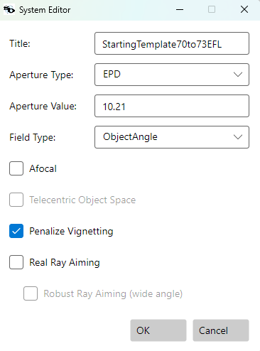
OpticalSystem.PenalizeVignetting is a system-level boolean (set in
the GUI's System Editor dialog, or via set_penalize_vignetting in
the MCP / CLI). When enabled, the engine overrides the off-axis
tolerance described above and applies the stiff per-ray penalty to
every failed ray, regardless of field — on-axis and off-axis alike.
PenalizeVignetting |
On-axis ray failure | Off-axis ray failure |
|---|---|---|
false (default) |
per-ray penalty fires | residual = 0 (tolerated) |
true |
per-ray penalty fires | per-ray penalty fires |
When to enable it:
- Stock-lens designs. The lens diameters are catalog-fixed. The optimizer must not "buy" aberration relief by quietly clipping the off-axis pupil — the as-built lens would vignette light the design has already used to compute its merit. Force it to design within the parts' apertures.
- Specifications that quantify illumination. Anywhere relative
illumination is a delivered property (machine vision, projection,
uniform-flux instruments), tolerating off-axis vignetting can mask
designs that meet the spot/MTF target but fail the photometric one.
Setting
PenalizeVignetting = truekeeps the optimizer from clipping rays; add anILLoperand on top of that only if the illumination value itself is part of the spec. - Any system whose pupil aperture is hard-fixed. Beam-shaping systems with externally-determined stops, microscope tube lenses facing a real iris, etc.
When to leave it disabled:
- Wide-angle imagers and most photographic lenses where corner vignetting at field edges is a known and accepted trade-off — the merit function is allowed to find designs that vignette the outermost rays to relieve coma or astigmatism.
- Early-stage architecture exploration where you're more interested in spot/MTF behavior at the field center and don't want vignetting penalties dominating the merit gradient before the design has converged on a shape.
PenalizeVignetting is an alternative to using merit operands as
vignetting controls — not a complement to them. Pick one:
PenalizeVignetting = true— the simplest path when lens diameters are fixed (stock-lens designs, hard-mounted apertures). No additional merit operands are needed to keep the design from clipping rays at field edges; the per-ray penalty does that directly. Operands likeILLare then only needed if relative illumination itself is a delivered specification — not as a vignetting guard.PenalizeVignetting = falsewith merit-operand vignetting control — use this when you want fine-grained control over which vignetting is acceptable. Add operands such asILL(relative illumination at a field) withMinbounds to prevent the optimizer from buying aberration relief by clipping the off-axis pupil. Other per-field operands can be combined to keep specific field zones unvignetted while letting outer edges roll off.
In short: check PenalizeVignetting and you don't need separate
vignetting-control operands. Leave it unchecked and you must add them
yourself, otherwise the off-axis vignetting tolerance described above
will silently let the optimizer earn merit by dropping rays.
Forbes (Rings × Arms) vs rectangular grid
The Forbes scheme places rays on Arms evenly-spaced radial spokes
at the Rings zeros of a Legendre polynomial in the area variable
ρ = r²/R². The rectangular scheme samples on a uniform Cartesian
grid and discards points that fall outside the unvignetted pupil.
Both estimate the same RMS integral; they differ only in how the
pupil is sampled and weighted.
Forbes is the default, and it should stay the default for almost
all design work. The reason is integration efficiency, not pupil
shape. For a smooth integrand — which any unvignetted, well-behaved
optical wavefront is — Gauss-Legendre quadrature converges
exponentially in the polynomial degree it can integrate exactly.
Forbes (1988) showed that for typical lens systems, ~12 rays of
Gaussian quadrature give 1% RMS-spot accuracy where ~75 rays of
the polar-uniform Andersen scheme are required, and a uniform
Cartesian grid needs roughly 500 rays for the same accuracy. In an
optimizer that evaluates the merit thousands of times per run, that
40× ray-count ratio dominates wall-clock time. Defaults of Rings = 6,
Arms = 12 generate 36 rays per off-axis field (Rings × Arms/2,
the Forbes half-arm convention — X-symmetry covers the rest) and just
6 rays on-axis (one per ring, by rotational symmetry) per
wavelength; both sit comfortably inside the regime where the residual
quadrature error is well below the visible aberration content. For
reference, a default 3-field (one on-axis) × 3-wavelength spot merit
expands to only ≈ (6 + 36 + 36) × 2 × 3 ≈ 470 operands — a small
fraction of what a dense rectangular grid costs (below), which is why
Forbes is the fast default.
There are, however, cases where the rectangular operands (SPOTR,
SPOTMR, WAVEXR, etc.) are the right tool:
Heavy or asymmetric vignetting. Forbes quadrature assumes a circular pupil; the Gauss-Legendre weights are derived for the full disk. When a substantial fraction of those weighted sample points fall in vignetted zones and are dropped, the remaining rays no longer carry the correct quadrature weights for the transmitted pupil. With only a handful of rings to begin with, losing two or three of them can bias the RMS estimate noticeably. A dense rectangular grid (e.g.,
GridSize = 16–32) over the same pupil degrades much more gracefully because each surviving ray still carries equal weight over its own grid cell — the loss is proportional, not weight-distorted. Forbes himself flags this in §3 of the 1988 paper: "for cases in which the effects of pupil distortion and vignetting need to be determined… simultaneously with the integration, pure Gaussian schemes are not possible."Aperture-defining variables (semi-diameter or CA %). When a surface's semi-diameter (Fixed mode) or clear-aperture percent (CA %) (Auto mode) is itself an optimization variable — for example, to trade image quality against vignetting (see Aperture variables in getting-started.md) — the transmitted pupil edge moves as the optimizer runs. With only a handful of Forbes rings, a boundary that sweeps across ring positions makes the merit respond to the aperture variable in coarse, quantized steps, and the Jacobian column for that variable turns noisy. A dense rectangular grid (
GridSize ≥ 64) samples the pupil edge finely enough that the merit — and its gradient with respect to the aperture variable — varies smoothly, so the LM step direction stays reliable.The maximum
GridSizeis 256 (any value you enter is clamped to the 4–256 range — the same ceiling as the spot-diagram analysis). The only real cost of a dense grid is that it traces more rays: a rectangular operand expands to two residuals (x and y) per in-pupil ray, for every field and every wavelength,operands ≈ 2 × 0.785 · GridSize² × N_fields × N_wavelengths≈ 1.57 · GridSize² · N_fields · N_wavelengthsso a
GridSize = 64grid over 3 fields × 3 wavelengths is ~58,000 rays per merit evaluation. Every optimizer path handles this — the default LM (finite-difference or analytic derivatives), the C# evaluator, and all the analyses evaluate grids up to the full 256 with no operand limit and no truncation. A denser grid simply takes proportionally longer; choose the density from the accuracy you need, not from any cap.On derivatives: with the analytic Jacobian (the optimizer default), a dense chief-referenced grid (
SPOTR,WAVEXR) evaluates about 1.8× faster than finite differences, while a dense centroid grid (SPOTMR) is roughly break-even (the centroid subtraction adds a second derivative pass). In absolute terms the analytic path evaluates a ~4,000-ray dense grid in tens of milliseconds — there is no dense-grid penalty beyond the ray count itself.Non-polynomial wavefronts. Strong aspheres, freeforms, or diffractive surfaces can produce wavefronts that aren't well approximated by a low-order polynomial in
ρ. Gaussian quadrature loses its accuracy advantage there; a denser uniform grid estimates the integral more honestly even if it costs more rays.Validation. When a Forbes-driven optimization converges to a surprisingly good merit value, re-evaluating the same design with a rectangular grid is a cheap independent check that the result isn't an artifact of the quadrature sample placement. If the two schemes disagree at the same total ray count, the design is probably exploiting structure the Gauss-Legendre points happen to miss.
In short: pick rectangular when you have reason to distrust the smoothness or circularity assumptions Gauss-Legendre is built on. Otherwise stay with Forbes — the speed difference matters more than it looks, especially on global-search and multistart runs.
Reference: G. W. Forbes, "Optical system assessment for design: numerical ray tracing in the Gaussian pupil," J. Opt. Soc. Am. A 5, 1943–1956 (1988).
Wavefront (OPD) Operands
RMS wavefront error over pupil quadrature, in waves.
| Type | Reference | Removed | Sampling |
|---|---|---|---|
WAVEX |
Chief ray | Piston and tilt | Forbes quadrature |
WAVEM |
Chief ray | Piston only | Forbes quadrature |
WAVEC |
Chief ray | Nothing | Forbes quadrature |
WAVEXR, WAVEMR, WAVECR |
same | same | Rectangular grid |
Inputs: Rings + Arms for Forbes; GridSize for rectangular.
The Forbes-vs-rectangular trade-off is the same as for spot
operands — see Forbes (Rings × Arms) vs rectangular grid above.
WAVEX is the standard diffraction-quality merit; the removed piston
and tilt prevent focus-shift and field-centroid shift from spuriously
driving the merit.
Ray-Intercept Operands
Single-ray queries. Evaluate at one (Surface, Wave, Hy, Px, Py).
| Type | Meaning | Unit |
|---|---|---|
RX, RY, RZ |
Ray position at surface | mm |
RL, RM, RN |
Ray direction cosines at surface | unitless |
AOID, AOIR |
Angle of incidence | degrees / radians |
AOED, AOER |
Angle of exitance | degrees / radians |
PX, PY, PZ, PL, PM, PN |
Paraxial equivalents of the above |
Inputs: Surface, Wave, Hy (normalized field 0–1), Px, Py
(normalized pupil -1..+1).
Angle Boundary Operands
Scan a surface range and report max/min angle of a chief ray.
| Type | Meaning |
|---|---|
RI |
Angle of incidence, degrees, across a surface range. |
RE |
Angle of exitance, degrees, across a surface range. |
Inputs: Surface1, Surface2. Typical use: set Max bound to
keep TIR margin on glass surfaces or to limit coating AOI.
Boundary Operands
Scan a surface range. Report min/max for use with Min/Max bounds.
Penalize the optimizer when outside the bound.
| Type | Meaning |
|---|---|
CV, CVA, CVG |
Curvature: all / air-only / glass-only |
CT, CTA, CTG |
Center thickness |
ET, EA, EG |
Edge thickness (at max SD) |
SD |
Semi-diameter |
DTRG |
Diameter-to-Thickness Ratio, Glass-only: `2·SD / |
Inputs: Surface1, Surface2 (range inclusive).
Glass-only variants walk only surfaces whose outgoing material is not air; air-only variants the complement; the plain variant both.
Total ("T") variants — sum every offending surface
Every boundary and angle operand above has a "total" counterpart, formed by
appending T to its name: CTT/CTAT/CTGT, ETT/EAT/EGT,
CVT/CVAT/CVGT, SDT, DTRGT, and RIT/RET.
Where the plain operand reduces a range to the single worst surface, a T
operand sums the bound violation of every qualifying surface in the range:
value = √( Σᵢ [ max(0, Min − vᵢ)² + max(0, vᵢ − Max)² ] )
It is 0 when every surface is within bounds, and grows as violations
accumulate. The residual is this aggregate against an implicit target of 0, so
you set Min / Max (the per-surface bounds) exactly as for the plain operand —
there is no Target to set.
Why use it. A worst-case operand only ever has a gradient on the one surface
that is currently worst, so the optimizer fixes offenders one at a time and can
stall when several surfaces violate at once. The T operand puts a gradient on
every offending surface simultaneously, which converges more smoothly when a
design drives many boundary constraints active. Same Surface1 / Surface2
inputs — reach for it wherever you'd use the plain operand but have several
surfaces to keep in bounds.
Model-glass total operands
NDT, VDT, DPGFT are T-style totals for the model-glass ("fictitious
glass") parameters — refractive index Nd, Abbe number Vd, and
partial-dispersion deviation dPgF. Each sums the Min/Max violation over the
model-index surfaces in the range (a real catalog glass has no such
parameter and is skipped). Use them to keep an optimized model-glass stack
inside a manufacturable index / Abbe / partial-dispersion box before you
substitute real catalog glasses. Inputs: Surface1, Surface2, Min / Max.
Surface sentinel values
Surface1 and Surface2 both accept either an absolute surface
index (positive integer — 1, 2, 3, …) or one of a small set of
negative sentinels. The same sentinel works identically in
either field — there is no separate "left-side" or "right-side"
sentinel set. Whichever endpoint you put it in, it resolves to the
position described below at evaluation time.
Use the sentinel form whenever the design will be edited by tools
(add_singlet, replace_element, split_element, surface insert/
remove) that shift the absolute indices — the sentinel auto-tracks
the renumbering, while a hard-coded positive index may end up
pointing at a different surface than you intended.
Sentinel values
| Value | Resolves to | Numeric position |
|---|---|---|
0 |
Mirror of whichever value you put in the other field | (depends on the other endpoint) |
-1 |
Surface immediately before IMG | Surfaces.Count − 2 |
-2 |
Image surface | Surfaces.Count − 1 |
-3 |
First surface after the stop | StopIndex + 1 |
-4 |
Stop surface | StopIndex |
-5 |
Surface immediately after OBJ | 1 |
A note on -5 and -1 — position-based, not material-aware
-5 and -1 are position sentinels: they always resolve to index
1 and Surfaces.Count − 2 respectively, regardless of what surface
type or material sits there. For a clean design where OBJ is followed
directly by the first glass-front and the last glass-back is followed
directly by IMG, these positions ARE the first and last refractive
surfaces — which is how they're commonly used.
Edge case to be aware of: if you've placed a dummy air surface
at index 1 (e.g. an explicit stop placeholder, a buried-pupil dummy,
or any other non-optical placeholder), -5 resolves to that dummy
surface, not to the actual first glass-front. Symmetrically, if a
trailing dummy sits between the last glass and IMG, -1 resolves to
that trailing dummy, not the actual last glass-back.
Example layouts:
| Layout | -5 resolves to |
-1 resolves to |
|---|---|---|
OBJ → L1 → L2 → L3 → IMG |
L1 front (✓ first refractive) | L3 back (✓ last refractive) |
OBJ → DUMMY → L1 → L2 → L3 → IMG |
DUMMY (the placeholder, not L1 front) | L3 back |
OBJ → L1 → L2 → L3 → DUMMY → IMG |
L1 front | DUMMY (the placeholder, not L3 back) |
If you have dummy surfaces in your design and want a span operand to
target the actual first / last glass-bearing surface, use the absolute
positive index instead of -5 / -1. (A material-aware "true first
refractive" sentinel is a planned future addition; for now, position
sentinels are what's available.)
Concrete examples
The same span operand CTA (center thickness, air-only) authored in
five common ways. Note that Surface1 and Surface2 are independent —
you can put a sentinel in either field, or both, or neither:
Surface1 |
Surface2 |
Resolved span | Meaning |
|---|---|---|---|
-5 |
-1 |
first refractive → last refractive | Every air gap between L1 and the last lens. Auto-tracks insertions/removals on either end. |
-3 |
-1 |
first surface after stop → last refractive | Every air gap from the lens after the stop to the last lens. Excludes everything on the front side of the stop. |
-4 |
-2 |
stop → image | Span starts AT the stop (covers the stop's trailing air) and ends at the image (covers the BFL gap). |
1 |
-1 |
absolute surface 1 → last refractive | Same range as (-5, -1) if your system has OBJ at index 0; if you later insert a surface at index 1, this hard-coded 1 will move with the renumbering only because SurfaceIndexUpdater shifts it — sentinel -5 is safer. |
5 |
0 |
absolute surface 5 → mirror of 5 | Just surface 5. The 0 "mirror" form is how you make a span operand evaluate at a single surface. |
You can also flip the order — the resolver normalizes the span so
s1 ≤ s2 after sentinel substitution. Surface1 = -1, Surface2 = -5
reads the same as Surface1 = -5, Surface2 = -1.
Where sentinels apply
Every boundary operand
(CT, CTA, CTG, ET, EA, EG, CV, CVA, CVG, SD,
DTRG) and every angle operand (RI, RE) shares the same Surface1
/ Surface2 semantics described above. So DTRG(-5, -1, max=10)
applies the diameter-to-thickness ratio constraint to every glass
element in the system without naming individual surfaces.
Where sentinels do NOT apply
Single-surface refs (the Surface column on WAVEX, EFL, BFL,
the Hy-driven distortion / lateral-color operands, and DM) take a
single absolute index. 0 on those fields means "system-level /
system default" — it is not a span-mirror sentinel because there's no
other endpoint to mirror.
Surface Property Operand
| Type | Meaning |
|---|---|
DM |
Diameter (= 2·semi-diameter) of one surface. Input: Surface. |
System Operands
Single value per system.
| Type | Meaning |
|---|---|
EFL |
Effective focal length |
MAG |
Paraxial lateral magnification |
AMAG |
Paraxial angular magnification |
ENPZ |
Entrance pupil Z (distance from surface 1) |
EXPZ |
Exit pupil Z (distance from image) |
ENPD |
Entrance pupil diameter |
EXPD |
Exit pupil diameter |
TTRACK |
Total track — surface 1 to image |
ILL |
Relative illumination at a field, = (F/#_axis / F/#_field)². Inputs: Hy, Arms (pupil-boundary direction probes — default 36, minimum 8). |
Optional input: Wave (defaults to primary wavelength).
First-Order Matrix and Parameter Operands
These read the paraxial ray-transfer (ABCD) matrix of the sub-system between two surfaces, or a stored surface parameter. They are the tools for lens synthesis — designing a real lens group to reproduce a target first-order matrix.
The sub-system matrix maps ray height y and geometric slope ω from the ray
incident on Surface1 to the ray exiting Surface2:
[y'; ω'] = [[A, B], [C, D]] · [y; ω]. Set Surface1 = Surface2 to read a
single surface's matrix.
| Type | Meaning |
|---|---|
A |
Element A of the sub-system matrix (Surface1 → Surface2). |
B |
Element B — units of length (mm). |
C |
Element C — units of 1/length (= −optical power). |
D |
Element D. |
DET |
Determinant A·D − B·C. A lossless group in a single medium has DET = 1 — target DET = 1 to keep a synthesized matrix physically realizable. |
Inputs: Surface1, Surface2, and optional Wave (defaults to primary).
| Type | Meaning |
|---|---|
PRMV |
Value of a surface parameter. Surface1 = the surface; Surface2 = the 1-based parameter index. |
PRMV reads the stored parameter selected by Surface2: the ABCD matrix
elements (1–4 = A, B, C, D), a Paraxial surface's focal length (1, in mm),
or an Even Asphere coefficient (1..N). A Standard surface has no parameters
(returns 0), and an out-of-range index returns 0.
Distortion and Lateral Color
| Type | Meaning |
|---|---|
DITAN |
Maximum signed F-tan(θ) distortion % across all fields. Reference is the paraxial EFL (or paraxial magnification for finite-conjugate object-height fields). |
DITHETA |
Maximum signed F-θ distortion % across all fields. Reference is the paraxial EFL. |
DITANF |
F-tan(θ) distortion % at a specific field. Input: Hy. Reference is the paraxial EFL. |
DITHETAF |
F-θ distortion % at a specific field. Input: Hy. Reference is the paraxial EFL. |
LCF |
Lateral color at a specific field — max chief ray height spread across all wavelengths. µm for focal systems, arcmin for afocal. Input: Hy. |
Sensitivity (As-Built Performance)
| Type | Meaning |
|---|---|
SENS |
Sum of ` |
The conventional design workflow optimizes nominal performance
first and then runs a separate tolerance analysis on top. SENS
folds tolerance sensitivity directly into the merit function. The
ray-bend at each surface — driven by (1 − cos θ) of the ray's
angle to the local normal weighted by the index step |Δn| — is
both the dominant aberration contribution and the dominant
sensitivity to fabrication errors (radius, thickness, tilt,
decenter). Adding SENS alongside the usual spot or wavefront
target steers the optimizer toward designs whose surfaces bend the
rays less aggressively, which means smaller perturbations under
tolerances. The as-built design may have slightly worse nominal
performance but holds up better through fabrication, and the
optimizer can land on different design forms entirely. Approach
follows Kenneth Moore, Photonic Instrumentation Engineering VI,
SPIE Proc. 10925, 1092502 (2019),
doi:10.1117/12.2508062.
Rings and Arms set a Gauss-Legendre pupil sampling identical to
the geometric MTF — start with Rings = 6, Arms = 12 and increase
only if the operand value looks noisy iteration-to-iteration.
Seidel Aberration Operands
These target the third-order (Seidel) aberration contributions directly. Each
returns the sum over a surface range (Surface1 → Surface2) of the same
per-surface coefficients the Seidel analysis reports — so a full-range sum
equals the analysis total, and a sub-range gives that group's partial sum.
| Type | Aberration | Seidel |
|---|---|---|
SPHS |
Spherical aberration | S1 |
COMAS |
Coma | S2 |
ASTGS |
Astigmatism | S3 |
FCS |
Field curvature (Petzval) | S4 |
DISTS |
Distortion | S5 |
ACS |
Axial (longitudinal) color | — |
LCS |
Lateral (transverse) color | — |
Inputs: Surface1, Surface2. There is no Wave input — the
monochromatic terms use the primary wavelength, and the color terms (ACS,
LCS) use the system's shortest and longest wavelengths.
Use these to balance a specific aberration across a chosen group of surfaces, or
to drive a term toward zero (e.g. FCS = 0 to flatten the field over the whole
lens). A flat plate in collimated light contributes zero to every Seidel term —
the operands only become non-zero where the rays are converging or the surfaces
have power.
Whole-system totals
The seven operands above take a surface range. Their T counterparts cover the
whole system and take no surface arguments:
| Span | Total | Aberration |
|---|---|---|
SPHS |
SPHT |
Spherical aberration (S1) |
COMAS |
COMAT |
Coma (S2) |
ASTGS |
ASTGT |
Astigmatism (S3) |
FCS |
FCT |
Field curvature / Petzval (S4) |
DISTS |
DISTT |
Distortion (S5) |
ACS |
ACT |
Axial (longitudinal) color |
LCS |
LCT |
Lateral (transverse) color |
A T operand returns exactly what the matching S operand returns over its full
range, and exactly what the Seidel analysis reports as the total — they share one
calculation.
Prefer the T form when you mean "the whole lens". A span authored as
Surface1 = 1, Surface2 = 8 does not widen when you insert a surface, so it
quietly stops covering the system it was written for; the T form cannot go
stale that way.
Fifth- and Seventh-Order Aberration Coefficients
Buchdahl/Rimmer coefficients, following Rimmer (1962). These are transverse coefficients scaled by the working F/number, and they need no ray tracing — which makes them practical for screening many candidate designs quickly.
Each comes in two forms: S sums over a surface range, T covers the
whole system.
| Span | Total | Aberration |
|---|---|---|
B5S |
B5T |
Fifth-order spherical aberration |
F1S |
F1T |
Fifth-order coma (first form) |
F2S |
F2T |
Fifth-order coma (second form) |
M1S |
M1T |
Oblique spherical aberration (first form) |
M2S |
M2T |
Oblique spherical aberration (second form) |
M3S |
M3T |
Oblique spherical aberration (third form) |
N1S |
N1T |
Elliptical coma (first form) |
N2S |
N2T |
Elliptical coma (second form) |
N3S |
N3T |
Elliptical coma (third form) |
C5S |
C5T |
Fifth-order astigmatism |
PI5S |
PI5T |
Fifth-order field curvature (Petzval) |
E5S |
E5T |
Fifth-order distortion |
B7S |
B7T |
Seventh-order spherical aberration |
Inputs: Surface1, Surface2 for the S forms; none for the T forms.
There is no Wave input — the primary wavelength is used.
The trailing
Shere means span, not Seidel. InSPHS…LCSit reads as Seidel, but fifth order is not Seidel, so the letter is reused with the plainer meaning.B5Sis "fifth-order spherical over a span", not "Seidel B5".
Aspheric surfaces are fully supported — conic constants and the A4, A6
and A8 even-asphere coefficients all contribute. Higher orders cannot reach
seventh order and are ignored: a deformation term in r^2m first contributes at
transverse order 2m − 1, so A4 reaches third order, A6 fifth and A8
seventh, while A10 and beyond start at ninth.
The A2 (r²) coefficient is not included in these coefficients, though it is
part of the surface sag everywhere else. If you use A2 on a surface, treat the
fifth- and seventh-order values for that surface as approximate.
Choosing a span
A surface's contribution to the fifth-order totals includes its induced
interaction with every surface ahead of it — that is inherent to the theory, not
an implementation choice. So a span beginning mid-system is well defined and the
spans still add up to the total, but such a value is not a property of those
surfaces in isolation the way a third-order span is. When in doubt, use the T
form.
PRMS — RMS Spot Size from the Aberration Coefficients
PRMS estimates the RMS spot radius at a field point directly from the
third-, fifth- and seventh-order coefficients above — no rays are traced. It
implements the analytic merit function of Robb, JOSA 66, 1037 (1976).
Because it costs a coefficient pass rather than a pupil of real rays, it is
substantially faster than SPOT. Speed is the reason to reach for it: the
ray-traced operands work perfectly well for the same searches, they simply cost
more per evaluation.
| Input | Meaning |
|---|---|
Hy |
Fractional field height at which the spot is estimated (0 = axis, 1 = full field). |
Wave |
Wavelength index, or blank for the primary wavelength. 0 means all wavelengths, combined using each wavelength's weight. |
The value is referenced to the centroid, as Robb's method specifies, not to the chief-ray intercept.
What it does not see
Three limits follow from what the coefficients are, and each one has bitten a real design:
It cannot see defocus. Every aberration coefficient is referenced to the paraxial image plane, so
PRMSreports the spot at that plane no matter where the image surface actually sits. A design can reach a lowPRMSwith a large real spot simply because the image plane is in the wrong place. Pin the plane with aPYoperand at the image surface targeted to 0, and add aBFLminimum so the focus cannot land inside the glass.It cannot see colour. Each wavelength is evaluated at its own paraxial focus, so axial and lateral colour do not appear in the value even with
Wave = 0. UseACTandLCTalongside it.It is a truncated series. The estimate is only as good as the orders it includes, so it degrades where the expansion does — at large aperture, large field, or on strongly aspheric surfaces.
It cannot see an aperture. The estimate is a closed-form function of the coefficients and the field height; no ray is traced, and no surface's semi-diameter or clear aperture enters it. A beam clipped at a surface — off-axis or on axis — produces the same value as one that passes unobstructed, and the vignetting penalty that the ray-traced operands apply never arises. Whether a design's apertures pass its beams is a separate question from what
PRMSreports.
Weighting it against the geometry
PRMS and the coefficient operands are numerically small next to boundary
operands like EG and EA, which are zero while satisfied and large when
violated. Starting from a poor design, a heavy image-quality weight can buy
spot size by driving the geometry negative — surfaces crossing before the rim.
Watch the edge-thickness operands as the tell, and raise image-quality weights
after the geometry is holding rather than before.
PRMSA — PRMS Over Every Field and Wavelength
PRMSA is a composite form of PRMS. One row expands, at evaluation time, into
one PRMS sub-operand for every combination of the system's fields and
wavelengths — a system with three fields and three wavelengths produces nine.
The expansion is fixed by the system, not by the operand:
| Fields | Every field in the field table. Each sub-operand's Hy is that field's height divided by the largest field height, so the set spans 0 to 1. |
| Wavelengths | Every wavelength in the wavelength table. |
| Weight | Each sub-operand carries PRMSA weight × field weight × wavelength weight. With all field and wavelength weights at 1, a PRMSA of weight w is nine PRMS rows of weight w. |
| Target | The PRMSA target, applied to each sub-operand. |
| Order | Wavelength-major: a wavelength's fields sit together. The coefficient set is monochromatic but field-independent, so one coefficient pass serves all of a wavelength's fields. |
Because the sub-operands are real operands, the least-squares structure is the same as writing them out by hand: the same number of residuals and the same Jacobian rows, not a single combined row.
Inputs it does not take
PRMSA has no Wave, no Surface, and no Rings/Arms:
Wave— it covers every wavelength, so there is nothing to select.Surface— likePRMS, it is a property of the whole system at a field point, not of one surface.Rings/Arms—PRMSevaluates Robb's integral in closed form over the pupil rather than by summing sampled rays, so there is no sampling density to set. The pupil average is exact to the truncation of the series.
What it does not see
Every limitation of PRMS applies unchanged to each sub-operand PRMSA
produces: defocus, colour, series truncation, and aperture clipping, including
on-axis clipping. See What it does not see above.
Arithmetic Operands
Derive new values from other operands already in the list. All operand
references are 1-based indices into the merit-function editor's
table (the number shown in the # column).
| Type | Meaning | Inputs |
|---|---|---|
MULTC |
Factor × Op1 |
Op1, Factor |
SUM |
Op1 + Op2 |
Op1, Op2 |
DIFF |
Op1 − Op2 |
Op1, Op2 |
MULT |
Op1 × Op2 |
Op1, Op2 |
DIV |
Op1 ÷ Op2 |
Op1, Op2 |
SUMR |
Σ Op[Op1..Op2] | Op1, Op2 (range) |
QSUMR |
√( Σ Op[k]² ) over Op1..Op2 | Op1, Op2 (range) |
DEV |
Σ ` | Op[k] − mean |
Target vs. Boundary Mode
Every operand can operate in either mode:
- Target mode — residual is
(value − target) × weight. Good when you want the value to equal something (e.g.EFL = 100). - Min/Max mode — residual is zero inside the bounds,
(value − min) × weightor(value − max) × weightoutside. Good for constraints like "CTG ≥ 2mm" where any value above the minimum is acceptable.
Switch via the Mode column. Target and bounds share the same numeric input field.
Tips
- Start simple. One
SPOTorWAVEXwith weight 1, plus a few boundary operands (CTG min,EG min,TTRACK max) is enough to optimize most classical designs. - Watch the displayed Value. After each evaluation the editor shows each operand's current value. If an operand is way off, check its inputs before assuming the optimizer is broken.
- Weights don't need to be normalized. LensHH-LT rescales pupil quadrature weights internally so that SPOT/WAVE contributions match their analysis-tool RMS values.
- Afocal systems. SPOT/SPOTM and lateral color automatically switch to angular units (arcmin) when the system is afocal.
Optimization
LensHH-LT ships three core optimizers — Local, Multistart, and Basin Hopping — plus two global modes: Global Multi Start Optimization (many Multistart restarts) and Global Evolutionary Optimization (a GPU-capable Differential-Evolution population search). All of them minimize the same merit function (see the Merit Function Reference) but differ in how they explore the variable space.
A typical workflow stages them:
- Search with Multistart, Basin Hopping, Global Multi Start Optimization, or Global Evolutionary Optimization when you don't trust the starting basin.
- Refine with the Local Optimizer once you're in the right basin.
- Polish with one more Local pass at the end so the final state is tightly converged.
Skip step 1 if you start from a known-good design; never skip step 3.
When to use which
| Optimizer | Good for | Not good for |
|---|---|---|
| Local (LM) | Refining a design you already trust — polish the last 10% of merit. | Escaping a bad starting point. |
| Multistart | Probing several random starts, LM from each. Cheap way to find a better basin and to vary glass choices. | Genuinely topology-changing exploration (it won't, e.g., find a Cooke triplet from a flat-plate start). |
| Basin Hopping | Heavy single-design exploration — the deepest one run can travel (can change topology). Random perturbations + Hooke-Jeeves pattern search + LM refinement, optionally with glass substitution. | Fast iteration — it's the slowest per run. |
| Global Multi Start Optimization | Surveying the solution space — collecting a gallery of distinct, locally-optimized design forms (different power patterns + glasses) to choose among, rather than one winner. | Driving a single design to its absolute lowest merit (use Local/Multistart). |
| Global Basin Hopping | The deepest single answer — many parallel Basin-Hopping (HJ+LM) chains that pool their best basin and reseed each stalled chain from the others' elite, running until you stop. The most thorough escape for one design when you can spend the compute. | Surveying many forms or quick iteration — it pours all chains into one answer (use Global Multi Start for a gallery) and is the most compute-intensive. |
| Global Evolutionary Optimization | Building a gallery of polished starting designs from a poor or power-free start (e.g. parallel plates) by evolving a whole population in parallel — GPU-accelerated. The fastest "no design → many viable forms" route. | Driving a single chosen design to its absolute lowest merit. |
Preview: what will actually run (new in 1.0.152)
Every optimizer dialog has a Preview button next to OK/Cancel. It reports what the run will do before you start it, and it is worth using whenever a run is slower or worse than you expected.
The reason it exists: the dialogs let you choose a merit engine and a derivative mode, but the optimizer silently overrides those for designs it cannot handle, and there was no way to see that it had. A run could sit on the slower path for a whole session with no indication.
Preview reports:
- the merit/Jacobian engine that will actually be used — C# or native C++, finite-difference or analytic;
- why, if it differs from what you selected — naming the variable or operand responsible;
- whether the GPU takes part, and if not, why not;
- the variable and operand counts, and whether the native engine loaded.
When the requested path cannot be used, the report says so and names the cause:
WILL RUN:  C# Finite-Difference (fell back from Native: model-glass variables)

Requested: Native Analytic

DOWNGRADED, because:
  model-glass variables
Preview asks the same code the optimizer uses to choose its path, so it cannot disagree with the run. It is disabled while a run is in progress.
The same query is available from the CLI as optimize preview, which accepts
engine=, analytic=, broyden= and gpuimage so you can test a
configuration before committing to it.
Why a run might not use the engine you picked
The native analytic path does not cover everything. These send a run to the C# finite-difference engine instead, and Preview names whichever applies:
| Cause | Note |
|---|---|
| Semi-diameter / clear-aperture variables | Their merit dependence is ray clipping, which the analytic Jacobian cannot represent. |
| Model-glass variables | No model-index support in the native batched path. |
| Paraxial power variables | Optimized in reciprocal (diopter) space. |
Ray-angle operands RI/RE/RIT/RET with analytic derivatives |
The native angle derivative diverges off-axis. |
Paraxial ray operands PY/PZ/PL/PX/PM/PN under a non-EPD aperture |
Their launch height is the pupil radius, which F/# and object-space NA derive from EFL. Under an EPD aperture these run native analytic. |
| Automatic vignetting factors | The per-field pupil remap exists only in the managed trace. |
Variables
The optimizer moves any parameter marked Variable in the Surfaces table. Typical choices:
- Curvatures (all or selective).
- Thicknesses (glass and/or air).
- Conic constants — available on every surface (the surface stays Standard until you set a non-zero conic; even-aspheres carry a conic in addition to the polynomial coefficients).
- Aspheric coefficients on even-asphere surfaces.
- Focal length of a Paraxial (ideal-lens) surface. You enter and read
the focal length in millimetres, but — exactly like Radius vs Curvature —
the optimizer varies the power (diopters,
1000/f). Power is what makes the bounds meaningful: it is continuous through afocal (f = ±∞ ↔ 0 D) and sign-symmetric, so aMin/Maxrange like−20 … 20 Dis well defined whereas a focal-length range spanning infinity is not. The variable is labelled Focal Power (D) in the editor. - Glass choice — Multistart and Basin Hopping can substitute glasses during search.
- Clear-aperture semi-diameter on Fixed-aperture surfaces — let the optimizer size the aperture directly, with automatic vignetting factors keeping the pupil sampling correct and an on-axis clearance floor protecting the axial beam. See Semi-Diameter as an Optimization Variable for the worked Cooke-triplet-with-vignetting case study.
Every variable carries optional Min / Max bounds. Internally the
LM solver works on an unbounded transformed variable, so the
bounds are never violated and the optimizer can't crash by trying
illegal values; the practical effect is that pushing against a
bound shows up as a vanishing gradient, not a hard wall.
Bound handling: Sigmoid or Reflect (new in 1.0.147)
That vanishing gradient is a real limitation, and you can now choose the
mapping that produces it. System → System Editor → Bound Handling offers
two modes; the setting is system-level (it applies to every optimizer — Local,
Multistart, Basin Hopping, the evolutionary searches) and is saved in .lhlt.
| Mode | Mapping | Behaviour at a bound |
|---|---|---|
| Sigmoid (default) | Scaled logit/sigmoid between the bounds | Smooth and monotonic, but the slope flattens toward zero as the variable approaches Min or Max. A variable pushed onto a limit effectively stops responding to the optimizer. |
| Reflect | The variable stays in physical units; out-of-range values fold back inside (a triangle wave) | The slope magnitude is always exactly 1, so there is no dead zone. A variable sitting on a limit keeps its full sensitivity. The cost is a kink in the derivative at each fold point. |
When to switch to Reflect. Use it on constrained problems — designs where several variables genuinely want to sit against their limits (edge and centre thickness floors, a maximum diameter, a bounded focal power). Under Sigmoid those variables go quiet one by one as they reach their bounds and the search loses dimensions it still needs; under Reflect they keep contributing. It also helps the stochastic searches, whose random kicks routinely land out of range.
Starting from a power-free design. A stack of flat plates, or any start with no real form yet, is the case where bounded thicknesses matter most. Left unbounded, the optimizer readily walks into negative centre thicknesses and crossed surfaces — geometry that cannot be built and that the search does not reliably come back from. Bounding the thicknesses makes those states unreachable rather than merely expensive, and Reflect is what keeps a variable responsive once it settles on one of those bounds.
When to stay on Sigmoid. Unconstrained or lightly constrained designs, where nothing spends time on a limit, gain nothing from Reflect — and Sigmoid's smoothness is friendlier to LM's quadratic model. Sigmoid remains the default so existing designs reproduce exactly.
Note. Variables with no
Min/Maxare unaffected: with nothing to fold against, both modes are the identity. If switching to Reflect changes nothing on your design, check whether your variables actually carry bounds — a design that constrains thicknesses withCT/CTA/CTGpenalty operands rather than variable bounds has unbounded variables, and bound handling does not apply.
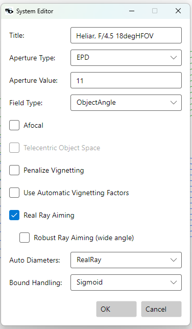
Outside the GUI: system set-bound-handling sigmoid|reflect in the CLI, and
set_bound_handling in MCP; system info reports the current mode.
See Getting Started → Your First Optimization for the GUI workflow of marking variables and setting bounds.
Local (LM)
Optimization → Local Optimizer
A damped-least-squares Levenberg-Marquardt solver — the workhorse of every modern lens optimizer. Each iteration:
- Compute the residual vector
rand JacobianJ(analytic where possible, finite-difference otherwise). - Solve
(JᵀJ + λI) Δx = −Jᵀ rfor the stepΔx. - Take the step if the merit improves and shrink λ; otherwise reject, expand λ, and retry.
This adaptive damping is what makes LM robust: when λ is large the step approaches gradient descent (safe but slow); when λ is small the step approaches Gauss-Newton (fast but only valid near the optimum). LM gracefully transitions between the two.
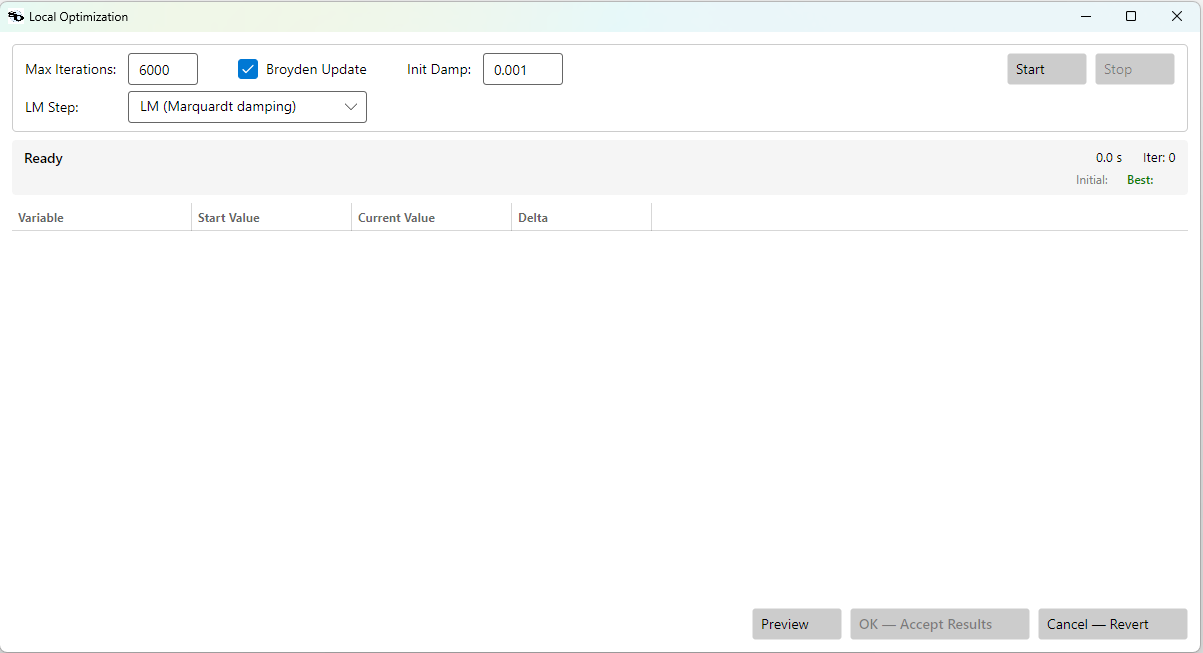
| Setting | Default | Meaning |
|---|---|---|
| Max Iterations | 4000 | Hard cap. The solver normally hits its tolerance long before this. |
| Use Broyden Update | on | Reuse a rank-1 Jacobian update between full finite-difference recomputes. A full J is rebuilt every 5 accepted steps; rejections reuse the existing J because x hasn't moved. The Broyden rank-1 step is applied only on accepts, using the actual old-x → new-x residual difference. Roughly 3–5× faster than a full Jacobian per step and matches results in almost all cases. Turn off if a run looks stuck or for very small systems where the speedup doesn't matter. |
| Init Damp | 1e-3 | Starting value of λ. The default is robust on aspheric mixes and well-conditioned problems alike. Drop to 1e-6 for gauss-newton-like behavior on very smooth, well-scaled designs; raise to 1e-2 if the optimizer keeps rejecting steps early. |
LM Step: damping or PSD (new in 1.0.150)
Step 2 above adds λ to every variable's diagonal term. That single number is standing in
for something that is not single: each variable's own curvature. In a real lens those
curvatures differ enormously — a nearly linear airspace and a strongly nonlinear surface
curvature can be many orders of magnitude apart — so whatever λ steadies the nonlinear
variable will throttle the linear one, and vice versa. The usual symptom is a run that slows
to a crawl, or reports convergence, while still some way from the minimum.
The LM Step control offers an alternative. Instead of one damping value, PSD (pseudo-second-derivative) estimates each variable's curvature directly and uses that on the diagonal. The estimate is nearly free: it comes from comparing the derivatives already computed on two successive iterations. PSD III is the stronger of the two variants offered; PSD II is the simpler earlier form.
| Setting | Default | Meaning |
|---|---|---|
| LM Step | LM | LM uses one damping value for all variables. PSD II / PSD III estimate per-variable curvature instead. |
Where the damping term really belongs. Damped least squares builds the normal-equation matrix as
L_jk = Σ_i (∂f_i/∂x_j)(∂f_i/∂x_k) + D² (on the diagonal, j = k)
The exact Gauss-Newton-plus-curvature matrix wants a second-derivative term in that same slot:
L_jk = Σ_i (∂f_i/∂x_j)(∂f_i/∂x_k) + Σ_i f_i ∂²f_i/∂x_j∂x_k
Dilworth's observation is that D exists only as a stand-in for that unknown
curvature — it occupies precisely the place where the second derivative should
be added — and that a usable estimate is already available for free: difference
the first derivatives of two successive iterations and divide by the step taken.
That is the PSD I method:
∂²f_i/∂x_j² ≈ ( ∂f_i/∂x_j |Δx_j − ∂f_i/∂x_j ) / ( Δx_j + ε )
PSD I needs the stabiliser ε, because a variable that barely moved on an
iteration yields an enormous spurious curvature and is then damped so hard it can
never move again. PSD II replaces that arbitrary constant with the step
actually taken by all the other variables — scale-aware and self-tuning:
∂²f_i/∂x_j² ≈ ( ∂f_i/∂x_j |Δx_j − ∂f_i/∂x_j ) / ( |Δx_j| + √(Σ_(k≠j) Δx_k²) )
PSD III goes further. The mixed partial is taken as roughly equal to the
homogeneous one, but that involves both j and k; the two are combined by the
ratio of the previous iteration's second-order terms, with
sec_j = Σ_i f_i ∂²f_i/∂x_j∂x_k evaluated at k = j:
∂²f_i/∂x_j² ≈ ( ∂f_i/∂x_j |Δx_j − ∂f_i/∂x_j ) / ( |Δx_j| + √(Σ_(k≠j) Δx_k² · sec_k/sec_j) )
This is why the benefit tracks variable count. The term that lands on the
diagonal now differs from one variable to the next by as much as fourteen orders
of magnitude, where classical DLS applies one constant D to all of them.
References.
- D C Dilworth, "Pseudo-second-derivative matrix and its application to automatic lens design", Appl. Opt. 17(21), 3372–3375 (1 November 1978).
- D C Dilworth, "Improved convergence with the pseudo-second-derivative (PSD) optimization method", Proc. SPIE 399, 159 (1983).
- D C Dilworth, Lens Design, appendix B.3 "The PSD methods" — the derivation above follows this account, which introduces PSD III.
When it helps. The benefit grows with variable count, because that is what widens the
spread of curvatures a single λ cannot cover:
| design | variables | outcome |
|---|---|---|
| Cooke triplet | 12 | no measurable difference |
| double Gauss | 21 | reaches minima 5–15% lower |
| conoscope | 93 | LM stalls; PSD III converges 9.9% lower |
On that conoscope the standard step with Broyden on reported convergence after 188 iterations at 6.71e-2 — it had stopped improving, not arrived. PSD III converged properly at 6.05e-2. PSD III also passed LM's final answer within about 50 iterations, so most of the gain arrives early.
Effect on glass substitution. A glass swap is a large, discrete jump that leaves the design far from its basin. On a 23-glass conoscope, substituting one glass raised the merit from 8.9e-2 to 1.08; PSD III recovered it within 50 iterations and finished better than the original design, while the standard step did not recover it at 50, 200, 800 or 2000 iterations. Where glass substitution matters, this can decide whether candidate glasses are ever accepted at all.
When it does not help. In Basin Hopping on smaller designs, PSD has performed worse than the standard step — reaching poorer minima with more hops rejected. It converges quickly to a nearby minimum, which is an asset when refining one design and a liability when a search depends on wandering. Treat it as something to try on large, stubborn designs, and compare against the standard step on your own work before adopting it.
Broyden. Selecting PSD switches Use Broyden Update off, because PSD compares derivatives from two successive iterations and a Broyden update is an approximation rather than a fresh computation. The checkbox updates to show this and you can turn it back on. In practice this costs less than it appears: on the conoscope PSD III needed roughly a third of the iterations the standard step needed without Broyden.
Init Damp under PSD. λ is still used, but only as a fallback — on the first iteration
before any curvature estimate exists, for variables whose estimated curvature is zero, and
to shrink the step after a rejection. Once curvature is engaged it has little effect.
Iteration budgets. Because PSD III converges in far fewer iterations, the large per-trial iteration counts used elsewhere (6000 in Basin Hopping) are usually unnecessary with it, and a much smaller budget buys many more trials for the same time.
The merit-change tolerance (1e-10) and damping bounds are handled internally — you don't normally tune them.
Run it twice. A single LM run can stop on a tolerance hit while the merit is still detectably decreasing on a fresh restart. Hit Start again from the result; the second pass either confirms convergence or shaves another few percent.
Two ways to keep thicknesses sane
The Local Optimizer has no built-in opinion about whether a glass thickness or air gap is physically reasonable — it will happily collapse or invert thicknesses to chase image quality unless you constrain them. There are two equivalent ways to do that:
- Merit-function operands —
CTG,CTA(per-surface-range centre thickness, glass and air), andEG,EA(edge thickness, glass and air). Each carries a Min/Max bound and a weight; the evaluator adds a smooth penalty when the bound is approached. - Per-variable Min/Max bounds — set on the variable itself in the surface table (Thickness Min / Thickness Max columns). The LM solver works on a transformed unbounded variable internally, so the bound is never violated; pushing against it shows up as a vanishing gradient, not a hard wall.
Both are demonstrated below on the same Cooke triplet starting
point (50 mm EFL, EPD 10, three fields 0°/14°/20°, three
wavelengths 0.48/0.55/0.65 µm). Sample files:
samples/UserGuide/LensFilesForManual/.
Starting point
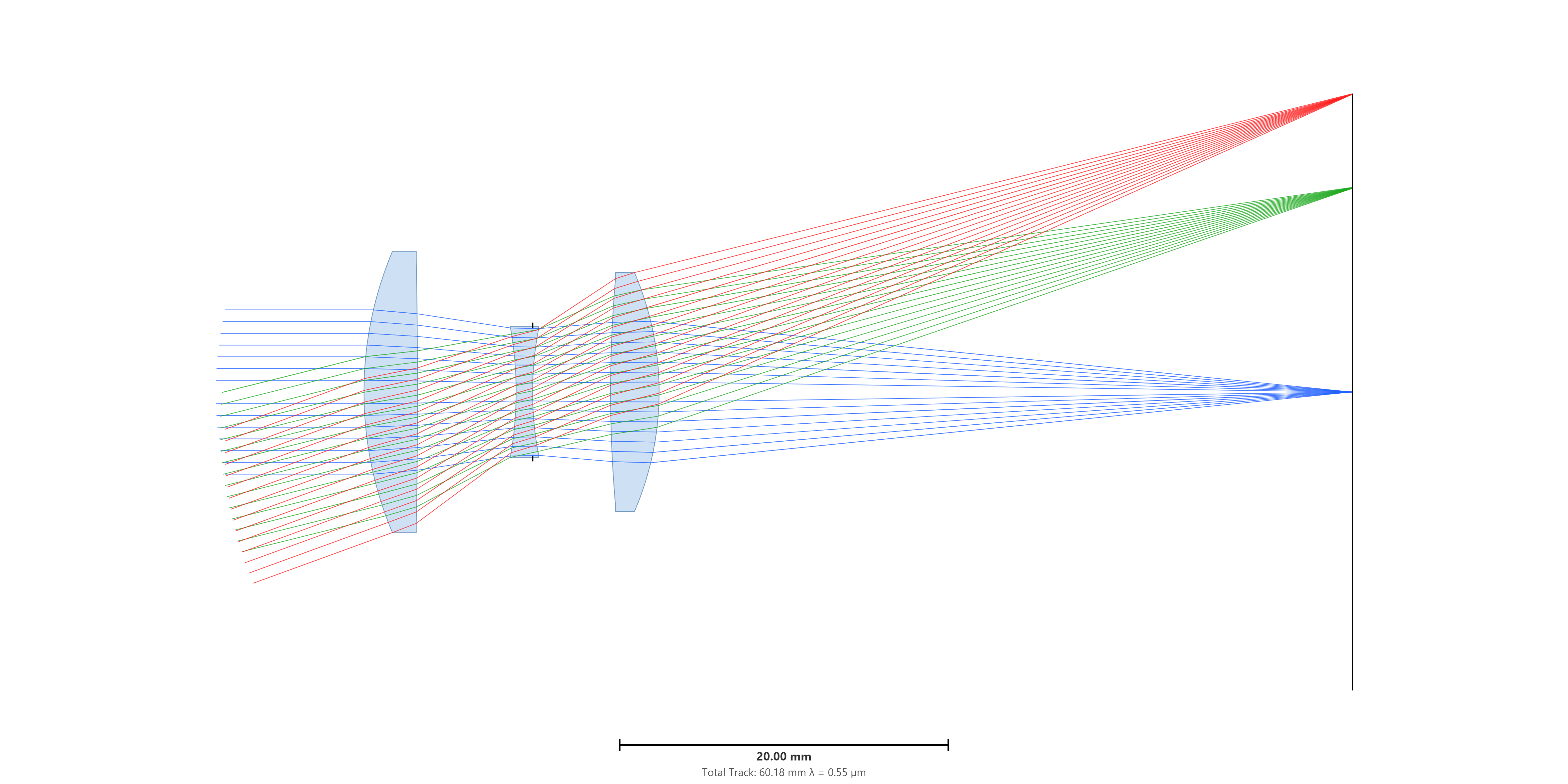
Variables are every curvature and every thickness from S1 through S6. The starting design is noticeably uncorrected:
| Spot — start | FFT MTF — start |
|---|---|
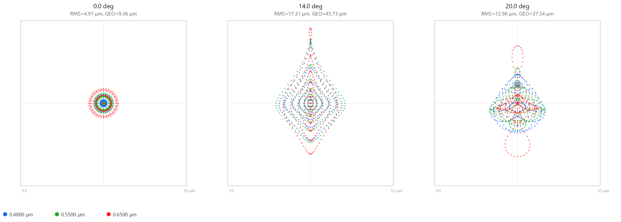 |
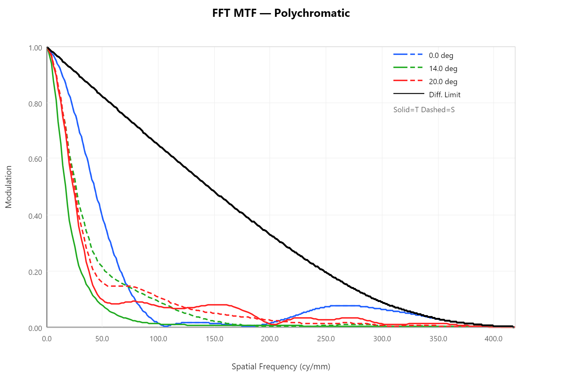 |
Case (a) — thickness handled entirely by the merit function
CookeTriplet_UC.lhlt. Variables carry no Min/Max bounds; the
merit function does all the work with EFL, WAVEX, CTG, CTA,
EG, EA, plus a CTA[6,6] Min=40 to keep BFL above 40 mm.

Convergence (133 iterations, 0.3 s):
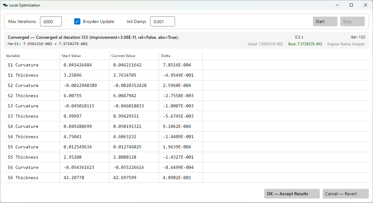
Merit goes from 0.0794 to 0.0757. Optimized layout:
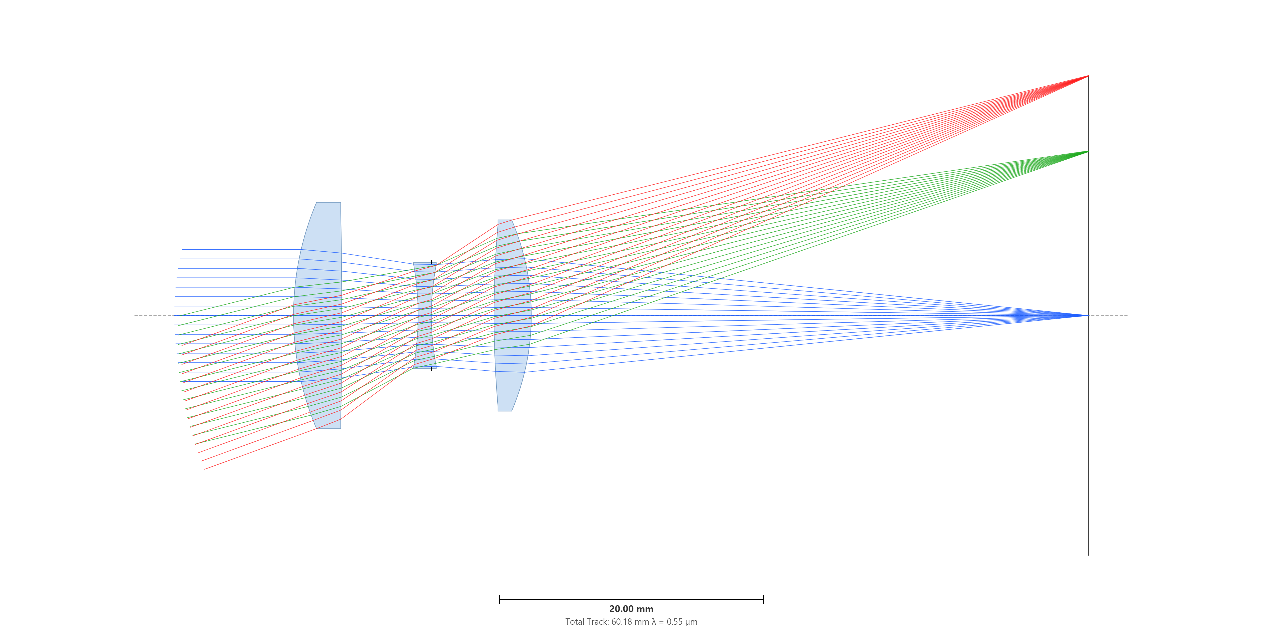
Case (b) — centre thickness handled by per-variable bounds, edges by merit function
CookeTriplet_C.lhlt. The merit function keeps only EFL,
WAVEX, EG, EA (edge thickness still belongs to the merit
function — there is no "edge" of a single variable). Centre
thicknesses are bounded directly on each thickness variable:
[1, 25] mm on glass thicknesses (S1, S3, S5), [0.1, 100] mm on
internal air gaps (S2, S4), and [40, 100] mm on the BFL (S6).

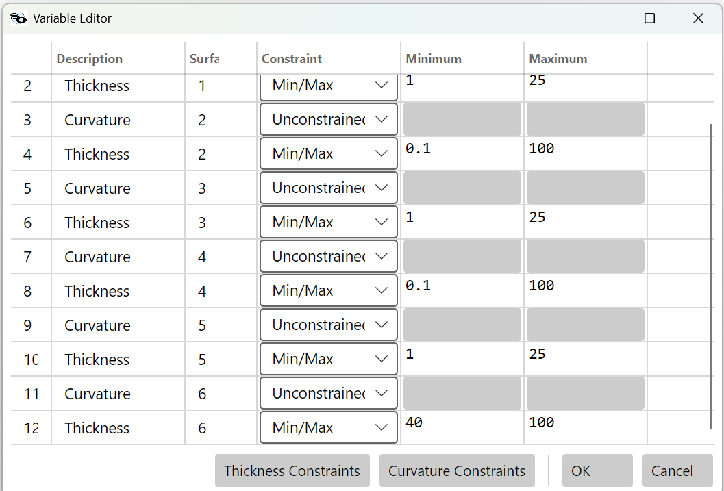
Convergence (566 iterations, 0.9 s):
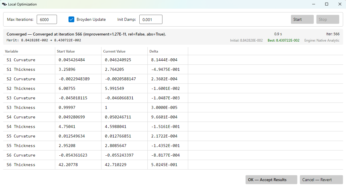
Merit goes from 0.0884 to 0.0843, and the optimized layout is
visually identical to case (a)'s — both constraint strategies reach
the same design. (The two merit values are not directly comparable:
case (a)'s merit also sums the CTG/CTA centre-thickness operands,
which case (b) replaces with variable bounds.) Constrained variables
take more LM iterations because the transform flattens the gradient as
a bound is approached — 566 here versus 133 for case (a), still well
under a second, though on a much larger system the gap can grow. Both
forms of constraint are supported; pick whichever fits your style.
Case (c) — no thickness handling at all
CookeTriplet_UC_NO_E_OR_CT.lhlt. The merit function has only
EFL and WAVEX; thickness variables have no bounds and no
boundary operands. The result is what you'd expect: the optimizer
collapses inter-element air gaps to negative values to overlap
glass elements, since that lets it bend rays more aggressively
without paying any penalty.
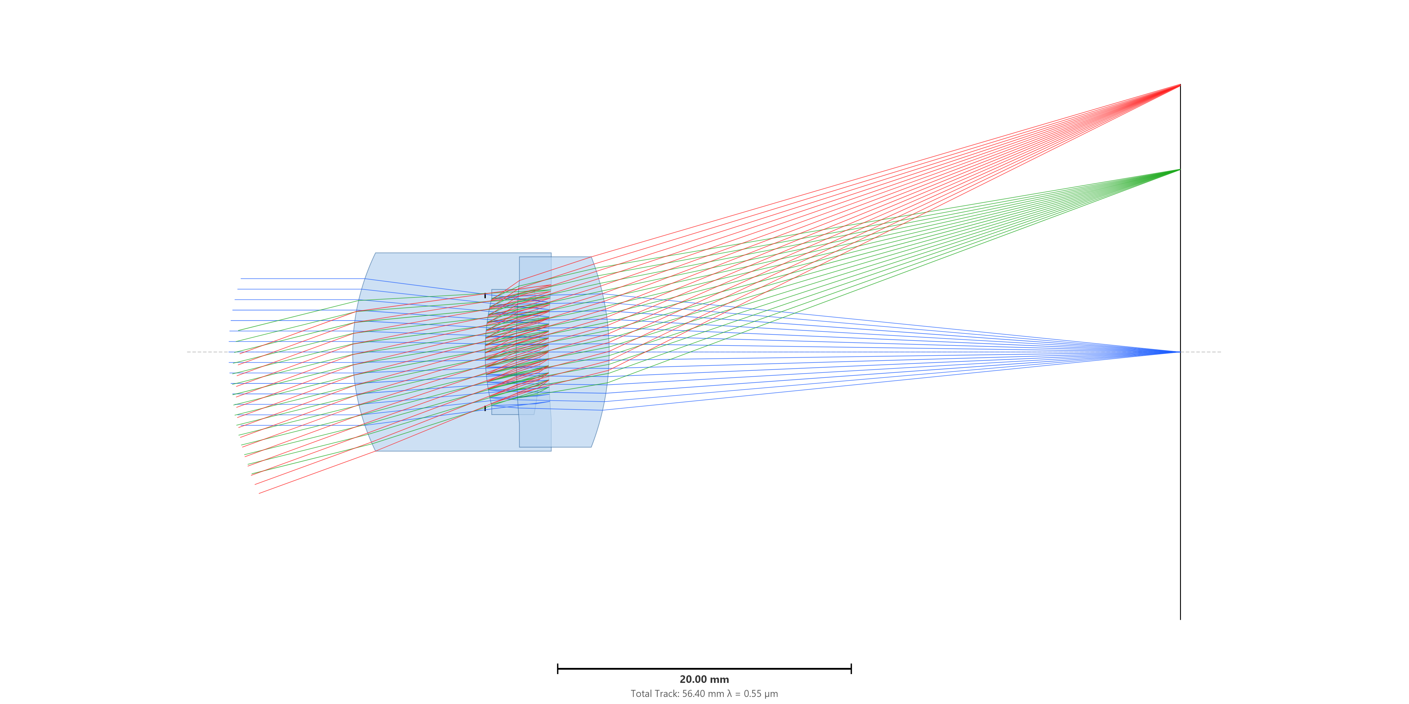
The reported merit is lower than (a) or (b), but the design is
physically meaningless — surface 2's air thickness comes out to
−0.58 mm and surface 3's glass thickness to −3.74 mm. Always
constrain thicknesses, by either of the two methods above, before
trusting an LM result.
Multistart
Optimization → Multistart…
Runs many LM optimizations from randomly perturbed starting points,
keeps the best, and tracks accepted vs rejected counts. Glass
substitution can be enabled — every trial may swap glasses on
substitution-eligible surfaces with a chosen probability. The
per-trial perturbation magnitude (Sigma) adapts during the run:
it starts small, grows when the search stalls (after several
consecutive non-improving batches, up to a cap) to climb out of a stuck
basin, and resets to its small starting value on every new best — so a
single starting Sigma covers a wide range of designs.
Algorithm at a glance
Two phases. Phase 1 runs one Initial LM polish from the user's
starting design — skip it (set Init LM = 0) when you already
trust the start. Phase 2 is the actual multistart loop: each
batch spawns N_CPU parallel trials, every trial perturbs around
the current center (a Metropolis random walk that is allowed
to drift away from best), runs HJ-LM polish, then competes for
acceptance. Successful trials reset σ to its small initial value;
when the search goes several consecutive batches without a new best,
σ grows one step (×1.5, up to the cap) to climb out of the current
basin — escalating exploration gradually as the search stalls.
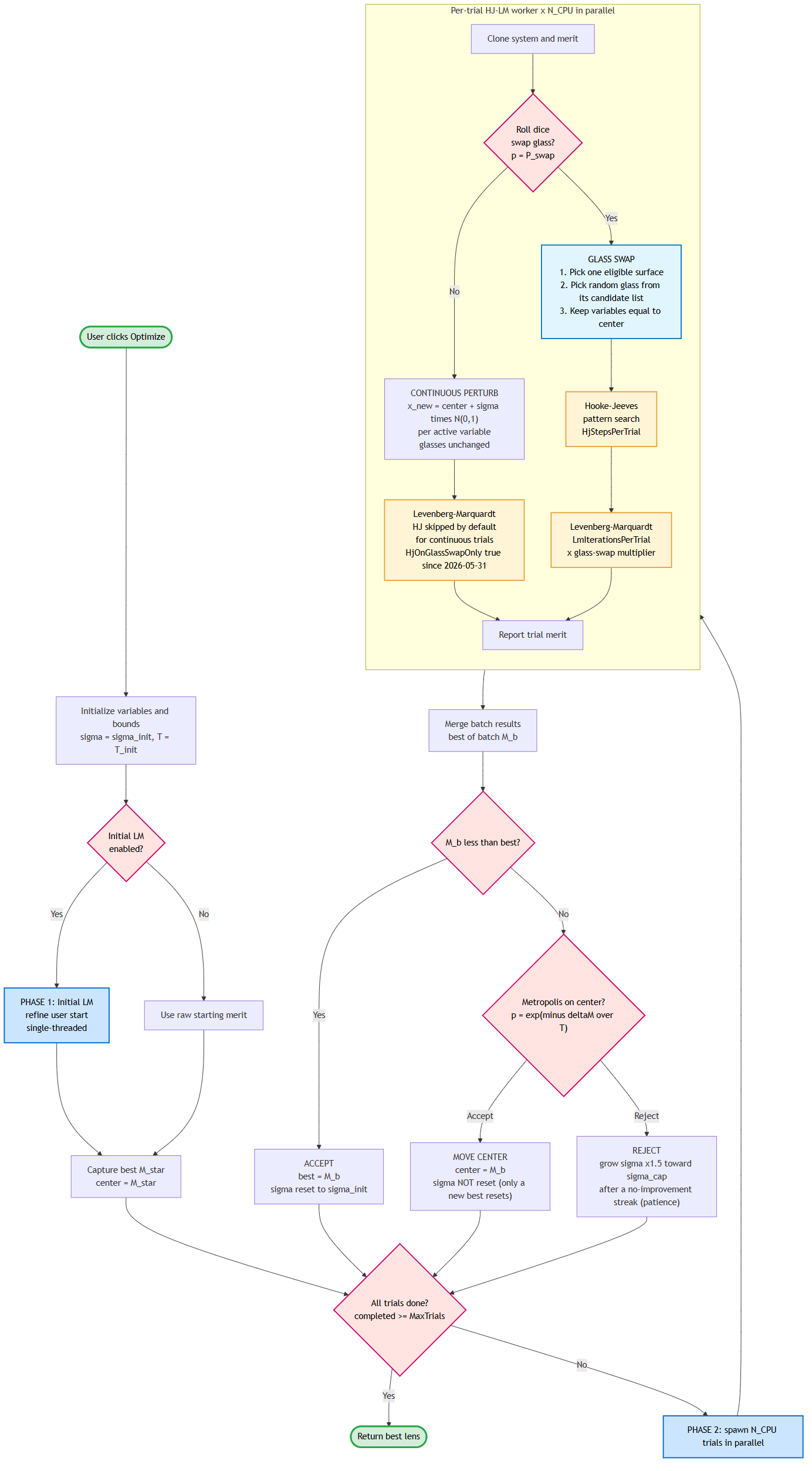
The HJ-LM atom (the Hooke-Jeeves and Levenberg-Marquardt steps in the per-trial block above) is
where each trial actually does its work. Hooke-Jeeves is a
derivative-free pattern search that climbs gracefully across
discontinuities (vignetting, ray-trace failures, glass-boundary
jumps); LM is the workhorse damped-least-squares solver that
polishes the basin once HJ has dropped you into it. By default
HJ runs only on glass-swap trials (LM's damping handles smooth
continuous perturbations on its own) — flip
HjOnGlassSwapOnly = false in the engine settings to restore the
pre-1.0.115 always-HJ behaviour.
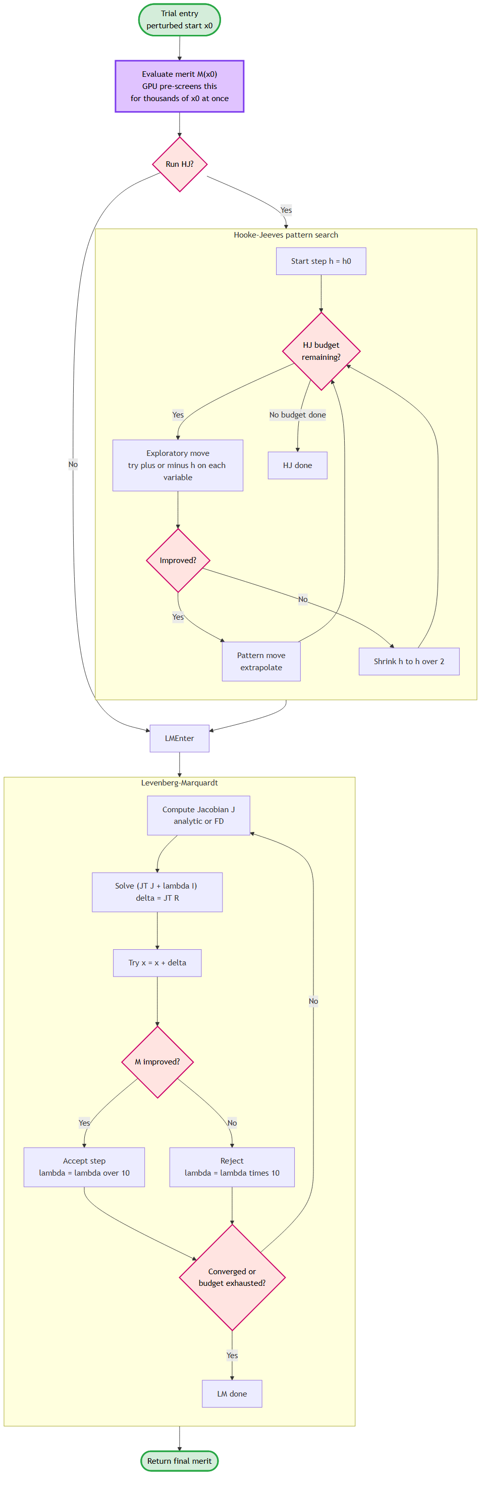
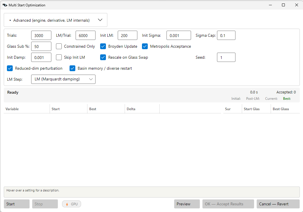
| Setting | Default | Meaning |
|---|---|---|
| Trials | 2000 | Hard cap on the number of LM optimizations. Stop earlier when satisfied. |
| LM/Trial | 4000 | Hard cap on LM iterations inside each trial. Per-trial wall-clock × Trials = total runtime budget. |
| Init LM | 4000 | One LM polish from the current design before the first random perturbation. Set to 0 to skip. |
| Init Sigma | 0.001 | Starting (and reset) value of the Gaussian-perturbation scale, relative to each variable's natural scale. σ starts here, grows on rejection toward Sigma Cap to escape, and resets here on every accepted improvement. The small default keeps each kick within LM's capture radius — it still escapes because σ grows when the search stalls. |
| Sigma Cap | 0.1 | Upper bound on σ — the largest kick the escape phase reaches. On a rejection streak σ grows ×1.5 per rejection up to this cap; any acceptance resets σ to Init Sigma. Raise it for wider exploration when refinement stalls. |
| Init Damp | 1e-3 | LM initial damping for every trial's per-trial LM run. Same meaning and default as the Local Optimizer's Init Damp. |
| Glass Sub % | 50 | Probability that a trial picks a fresh random glass for each substitution-eligible surface. 0 = never; 100 = every trial. The pool comes from the per-surface Glass Substitution Settings (each surface can draw from a different filtered catalog) — see Glass Substitution During Optimization. |
| Rescale on Glass Swap | on | When a glass is swapped, also rescale that element's curvatures by (n_old−1)/(n_new−1) so its optical power is preserved to first order — keeps the swapped design feasible instead of broken, which improves the typical (median) result. Only has any effect when glass substitution is active (Glass Sub % > 0 with substitutable surfaces); on fixed-glass designs it is a no-op. (Basin Hopping keeps this off — its small-step trajectory is over-perturbed by the per-swap curvature jump.) |
| Constrained Only | off | If on, only perturb variables that have Min/Max bounds. Useful when you want unbounded variables held fixed (e.g., a fixed-radius element). |
| Broyden Update | on | Same meaning as for Local LM. Leave on. |
| LM Step | LM | Same meaning as for Local LM: PSD II / PSD III estimate per-variable curvature instead of using one damping value. Worth trying on designs with many variables, and where glass substitution matters. Selecting PSD turns Broyden Update off. |
| Seed | 1 | RNG seed for the run. The same seed with the same settings and the same starting design reproduces a run exactly — which is what makes it possible to change one setting and attribute the difference to that setting rather than to luck. Change it (1, 2, 3, …) for a genuinely independent run. Caveat: the GPU pre-screen draws its candidates from an unseeded generator, so runs with the GPU sieve enabled are not reproducible even with a seed set. |
| Metropolis Acceptance | on | When on, Multistart keeps a current centre state separate from best and may accept a worse-than-best trial as the next centre with probability exp(−ΔM/T) (T autotunes from early |ΔM| samples). Lets the search walk out of basins it has already mined. Best is always strict-improvement; the returned design is monotone. |
| Reduced-dim perturbation | on | About half of trials perturb only a random subset of the variables — up to roughly a third of them — leaving the rest at their centre values, instead of kicking every variable at once. A full-dimension kick is usually pulled straight back to the same basin by LM; moving along these lower-dimensional manifolds lets the search slip into adjacent basins a full kick overshoots. |
| Basin memory / diverse restart | on | Keeps an archive of the distinct minima the walk has visited. Once sigma has saturated at the cap for several batches with no new best, the walk restarts from a fresh point chosen to lie far from every archived basin (with its glasses randomized), systematically mapping new regions instead of circling the same minimum. The run-wide best is tracked separately and is never lost — it, not the current region's best, is the reported answer. |
Convergence levers. The last three rows — Metropolis Acceptance, Reduced-dim perturbation, and Basin memory / diverse restart — are the convergence levers, all on by default. Together they turn Multistart from independent small kicks into a memory-guided walk that reaches deeper basins; leave them on unless you are deliberately reproducing the older kick-and-polish behaviour, in which case turn all three off.
Multistart's strength is variability — it's the cheapest way to sample several glass sets and several nearby basins with only modest perturbations. With the small default Init Sigma = 0.001 it isn't designed to flip a topology (a positive-power element won't become a negative-power element) in a single kick; for that, raise Sigma toward the cap, or use Basin Hopping.
Aspheric coefficients are perturbed with a per-order natural
scale rather than a single sigma applied uniformly. The natural
magnitude of an even-asphere term drops by y² per order
(A4 ≈ 10⁻⁶, A6 ≈ 10⁻⁹, A8 ≈ 10⁻¹², …) where y is the surface
semi-diameter, so a uniform sigma would kick A8 by orders of
magnitude more than its natural scale and produce NaN ray traces.
Multistart instead uses a per-coefficient reference scale of
1e-3 / y^(2(k+1)) for the k-th term and applies sigma
relative to that scale. Bounded aspherics (both Min and Max
set) use the bound-width-relative scale shared with the other
bounded variables; unbounded aspherics use the per-order rule.
Either way the perturbation magnitude tracks the term's natural
scale and an unbounded aspheric is now an honest variable in
Multistart, not a hold-current placeholder.
GPU pre-screen (Beta, new in 1.0.115; tuning knobs added 1.0.128)
Most random perturbations produce designs that are strictly
worse than the current best — running the full HJ-LM cycle on
them is wasted work. The GPU pre-screen filter, available
when LensHH-LT detects a CUDA-capable NVIDIA GPU, evaluates a
much larger candidate pool than N_CPU in a single GPU launch
(~60 µs per design on an RTX 4060), ranks by merit, and feeds
only the top survivors into the parallel HJ-LM workers.
Discarded candidates pay one merit evaluation each instead of
the 50–300 LM iterations a full trial would cost.
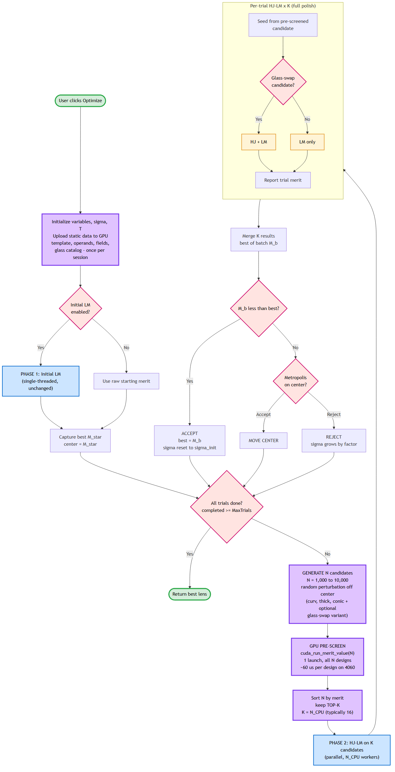
How to enable. Since 1.0.138 the pre-screen is a global setting rather than a per-dialog checkbox:
- Tick
Multistart GPU pre-screen (Beta)under Editors ▸ Preferences ▸ GPU acceleration. Multistart and Global Multi Start both read it, so every restart of a gallery search inherits the same sieve — see GPU Acceleration. - With no CUDA device the whole GPU acceleration group in Preferences is disabled and the status line above it says why.
- Every optimizer dialog carries a live ⚡ GPU status chip, so you can confirm at a glance that work is reaching the device.
- If your design uses aspheric, FieldY, or ConfigValue
variables the GPU kernel cannot accept it — it takes only
curvature, thickness, and conic coefficients per design. The run
falls back to the CPU path and the result line reports
GPU pre-screen requested but inactive (non-supported variable types (aspheric/field/config)).
Tuning the sieve (1.0.128). Two knobs turn the pre-screen
from a refiner into a basin-escape tool. The GUI runs them at
their defaults (2 % and 1×); the CLI and MCP expose both, and the
CLI also turns the sieve on per-run (optimize multistart … gpu mincurvchange=5 gpufill=10), as does MCP via useGpuPreScreen:
Min change (%)(CLImincurvchange=, MCPgpuMinCurvatureChangePercent) — the difference gate plus the survivor-distinctness threshold. A candidate is only worth GPU-evaluating if it is structurally different from the running best: a glass swap (|Δn_d| > 0.001) or a refractive surface whose curvature moved by more than this percent (a previously-flat surface gaining any curvature counts). The same threshold also keeps the surviving designs apart from each other, so a bigger pool spreads across the feasible region instead of collapsing onto the lowest-merit point. Survivors are still ranked by merit.0disables the gate. Default 2 %; values around 5–10 % give the most aggressive escape.Population ×(CLIgpufill=, MCPgpuPreScreenFill) — the sieve evaluates this many times the GPU's device-fill candidate count per batch (default 1 = one device fill, ≈6,000 designs on an RTX 4060). The GPU is otherwise idle, so a larger pool — e.g. 10× — is a near-free way to give the value-only sieve more shots at a design that polishes well under LM. Scales GPU kernel time and device scratch roughly linearly; if it runs out of GPU memory it falls back to CPU for that batch.
What runs on the GPU. Each Phase-2 batch generates a
device-filling candidate pool (Population × × device fill),
mixing continuous perturbations and — when glass substitution
is on — single-surface glass swaps in the same launch. The
whole-merit kernel computes the merit of every candidate
bit-equal to the CPU path; the difference gate forces each
candidate to clear Min change (%), and diversity-aware
selection then keeps the best N_CPU distinct survivors for
HJ-LM polish. Acceptance / Metropolis / sigma schedule are
unchanged. The GPU base design (curvatures and glasses)
tracks the Metropolis centre, so the sieve always scores
exactly the design the LM worker reconstructs.
Performance. On real production-class merits (Tanabe, 21-surface, 3 waves, 3 fields, 241 operands) the consumer-class RTX 4060 delivers ~1.7× the raw merit-evaluation throughput of a 16-thread laptop CPU. The pre-screen's wall-clock impact is larger because most candidates would have failed HJ-LM anyway: discarding them at ~60 µs each instead of running a 50–300-eval HJ-LM cycle compounds the 1.7× hardware win into a far bigger algorithm-level speedup. A100-class FP64 GPUs project to ~10–25× over the same CPU baseline.
Result message telemetry. When a run uses the GPU
pre-screen, the result line at the bottom of the dialog adds
| GPU pre-screen: N candidates sieved across M batches,
followed by a GPU↔CPU parity gap (≈0 confirms the sieve
scored exactly the design LM polishes) and a survivor spread (worst survivor merit + mean change from best — if
this is near zero the survivors are hugging the merit floor and
LM has little to do). When glass substitution is on, it also
reports how many of the HJ-LM survivors were glass-swap
candidates.
Multistart on the Cooke triplet
Sample file:
samples/UserGuide/LensFilesForManual/CookeTriplet_UC.lhlt — the
same 50 mm EFL triplet from the Local Optimization section (EPD 10,
three fields 0°/14°/20°, three wavelengths), every curvature and
thickness variable, thicknesses kept physical by the merit function
(CTG/CTA/EG/EA). Its starting merit is 0.0794. Where the
local optimizer only polished it to 0.0757, Multistart's random
restarts can jump out of that basin entirely.
Three scenarios show what that buys you — all from the defaults (Trials 3000, LM/Trial 6000, Init Sigma 0.001, Broyden and Metropolis on).
Fixed glass — curvatures and thicknesses only
With the glasses held fixed, Multistart perturbs only the continuous variables, and finds a basin far deeper than the local polish reached:
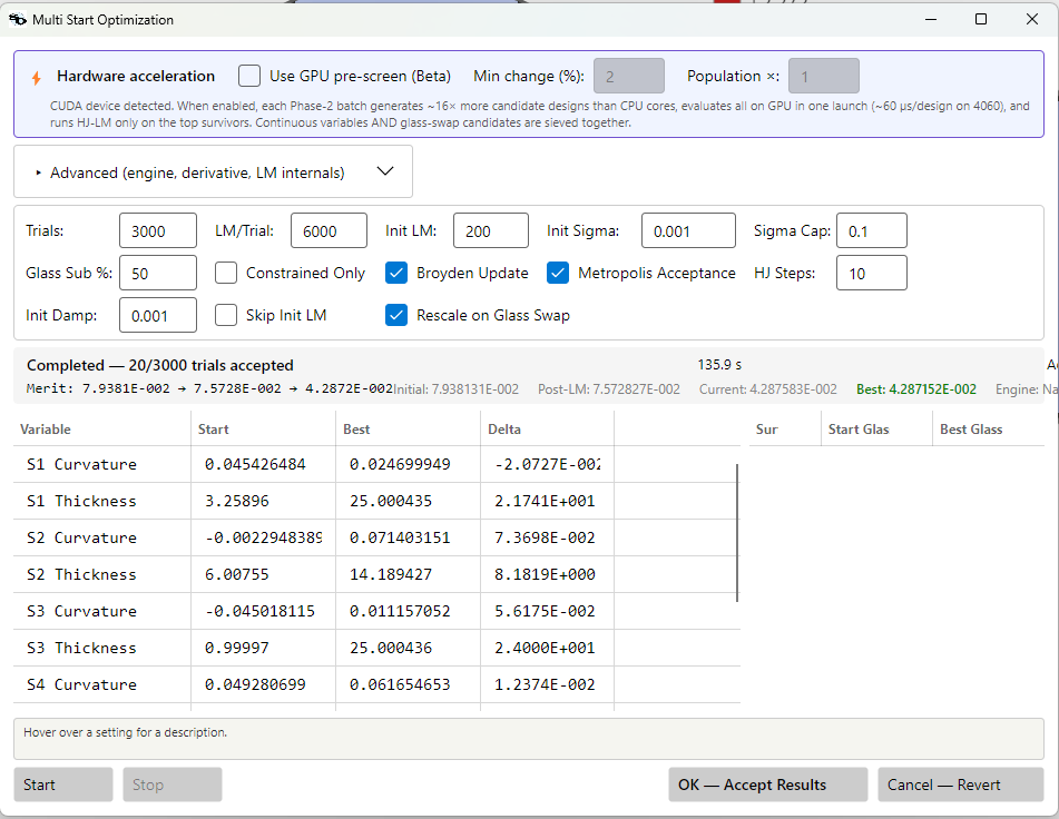
Result: 0.0794 → 0.0429 (136 s, 20 of 3000 trials accepted) — a ~1.85× improvement the local optimizer could not reach, because it was trapped in the starting basin.
| After — wavefront | After — FFT MTF |
|---|---|
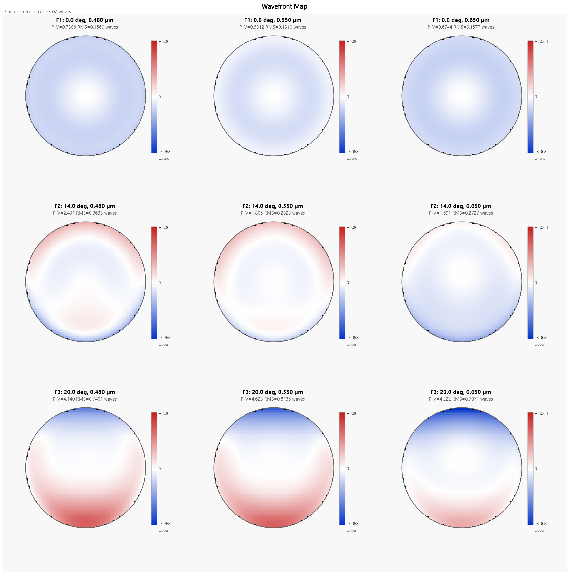 |
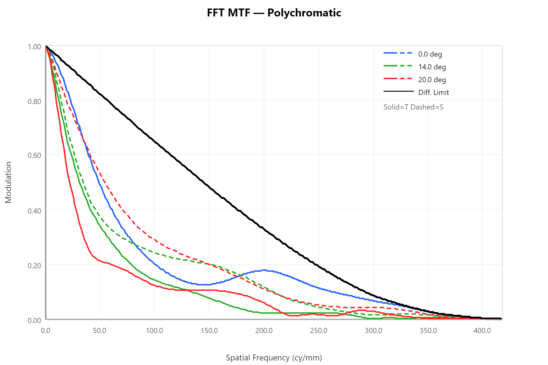 |
Glass substitution on
Letting the optimizer re-choose the three glasses from the CoreSet28 filtered catalog opens up more of the design space:
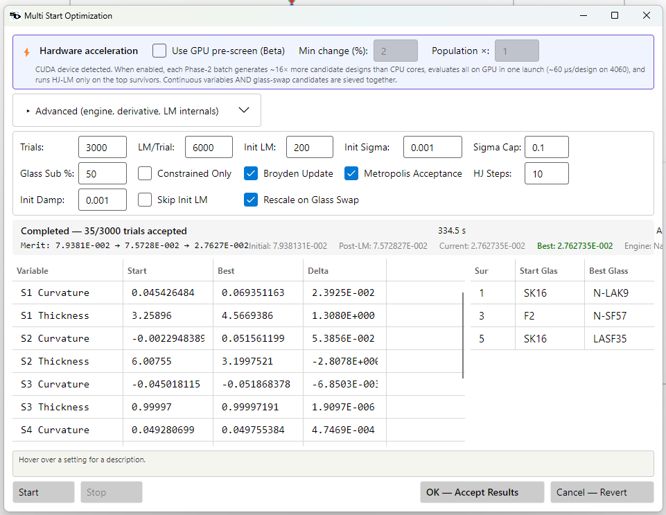
Result: 0.0794 → 0.0276 (335 s). The substitution replaced the starting Schott triplet with a set the search chose on its own:
| Surface | Start glass | Best glass |
|---|---|---|
| 1 | SK16 | N-LAK9 |
| 3 | F2 | N-SF57 |
| 5 | SK16 | LASF35 |
| After — wavefront | After — FFT MTF |
|---|---|
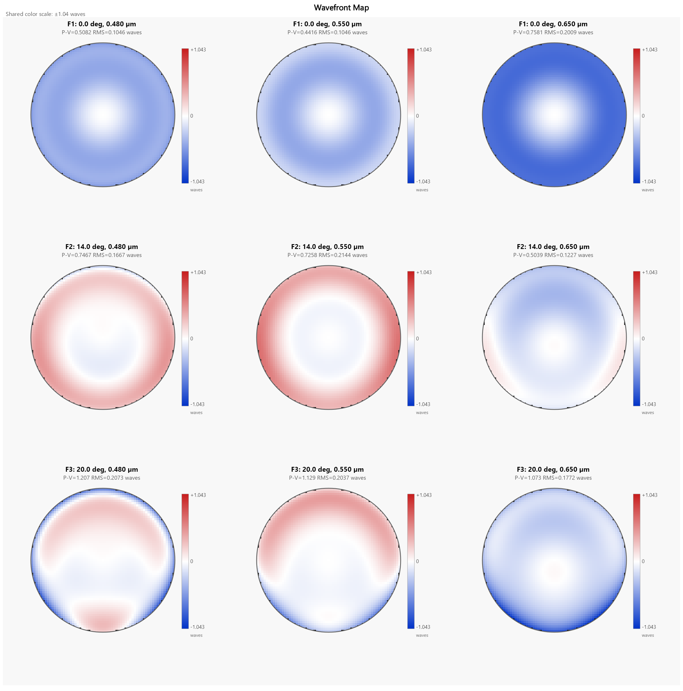 |
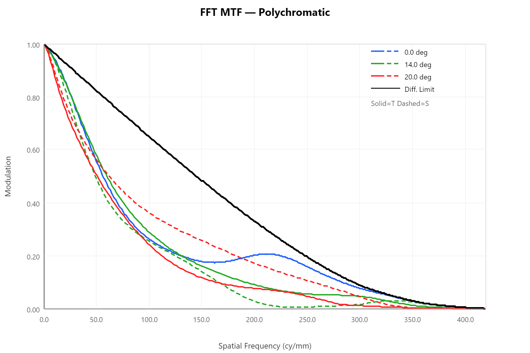 |
From a bare parallel plate
Multistart does not need a working lens to start from. Handed three flat plates — every radius infinity, no optical power — it rebuilds a real triplet:
| Before — three flat plates (merit 8.0 × 10¹⁴) | After — Multistart triplet |
|---|---|
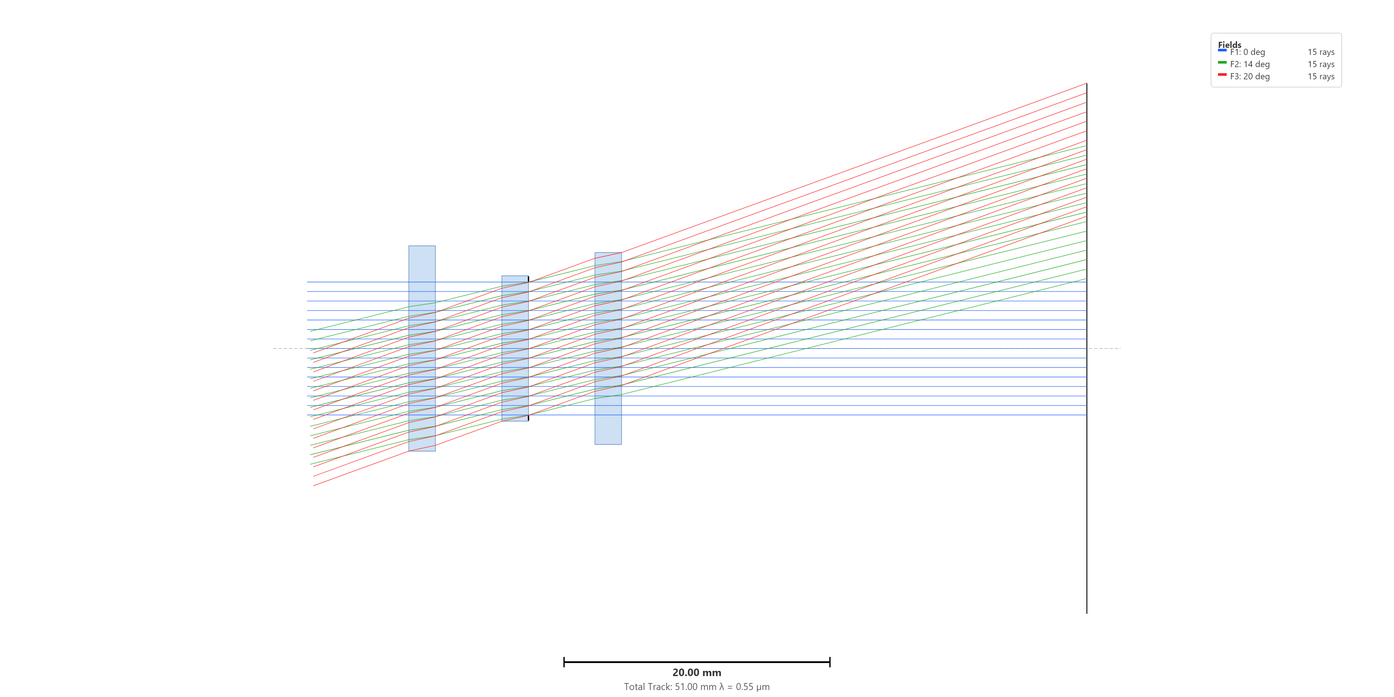 |
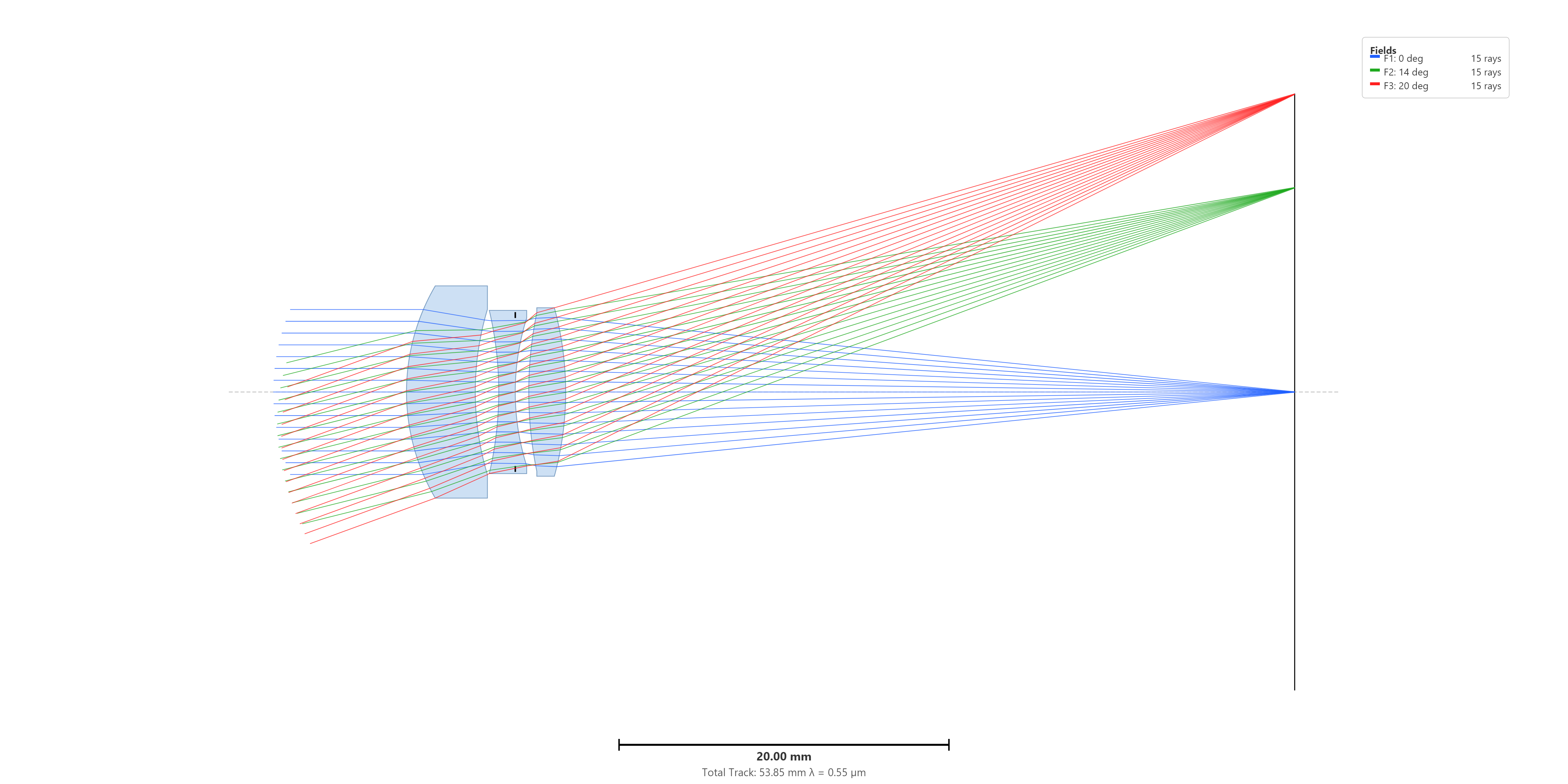 |
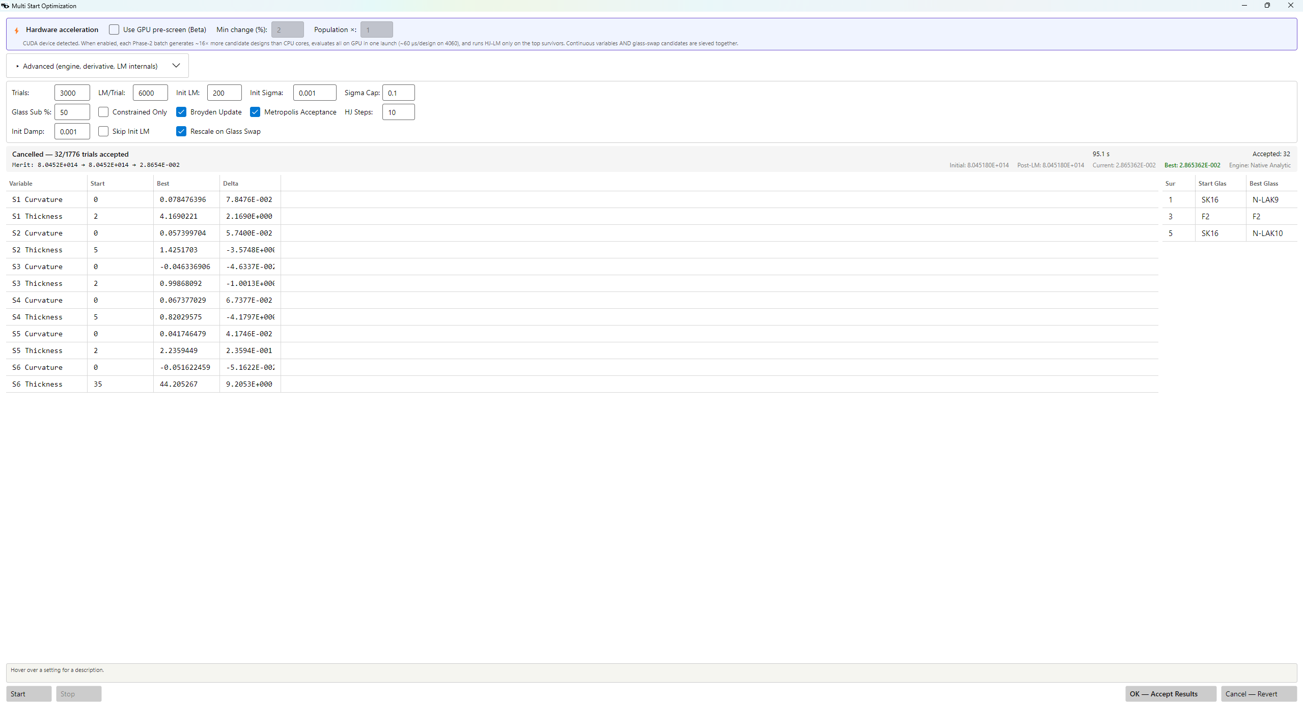
Result: 8.0 × 10¹⁴ → 0.0287 (95 s). Read the header carefully: the Phase-1 initial LM left the merit at 8.0 × 10¹⁴ untouched — a zero-curvature plate has no gradient for LM to follow — so every bit of progress came from the random restarts. Notice too that Multistart settles near ~0.028 from both the finished triplet (0.0276) and the flat plate (0.0287): consistent, but it lands in the same moderately-deep basin either way. Basin Hopping, next, digs deeper from the identical starts.
Init Sigma. These runs all use the default 0.001. The per-hop kick is small, but the LM refinement that follows amplifies it, and with Rescale on Glass Swap (on by default) keeping swapped designs feasible, 0.001 escapes basins readily here. If a converged design refuses to move, raise Init Sigma toward the cap (0.01–0.1) before deciding it is done for the chosen topology.
Global Multi Start Optimization
Optimization → Global Multi Start Optimization…
(Named "Global Search" before 1.0.122.)
Where Multistart returns the single best design it found, Global Multi Start Optimization returns a gallery of structurally-distinct, locally-optimized designs — so you can compare genuinely different solution forms (different element power-sign patterns, different glass sets) and choose the one that best suits your manufacturing and packaging constraints, not only the one with the lowest merit.
It runs many independent Multistart restarts from your starting design and keeps a result only if its lens form is new. Designs are de-duplicated by a form signature — the glass set plus the per-element power-sign pattern — so the gallery fills with distinct forms rather than many near-copies of the same basin. The gallery is sorted best-merit-first.
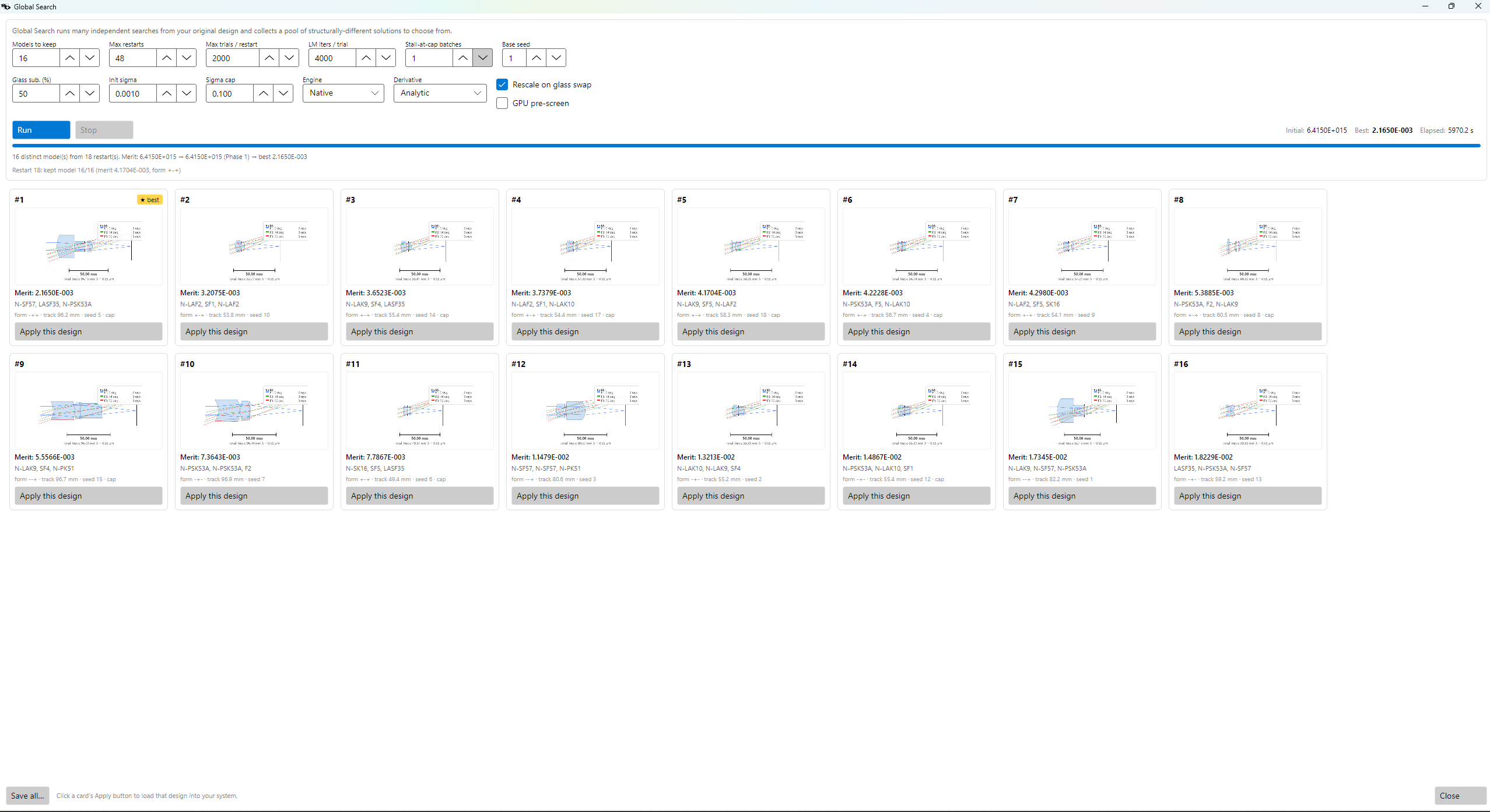
Algorithm at a glance
Phase 1 runs one deterministic LM polish from your starting design (call it
D0); it is computed once and seeds every restart. Phase 2 then runs
independent restarts: restart i is a full Multistart run from D0 with seed
BaseSeed × 100000 + i, so the restart batches never overlap and the whole
search reproduces from a single base seed (base seed 1 → 100000, 100001, …;
base seed 2 → 200000, …). After each restart converges, its best design's form
signature is computed; if that form is already in the gallery (within a small
merit tolerance) the restart is discarded as a duplicate, otherwise it is kept.
The search stops when it has collected Models distinct forms, exhausted
Max Restarts, or stalled (no new distinct form for several restarts).
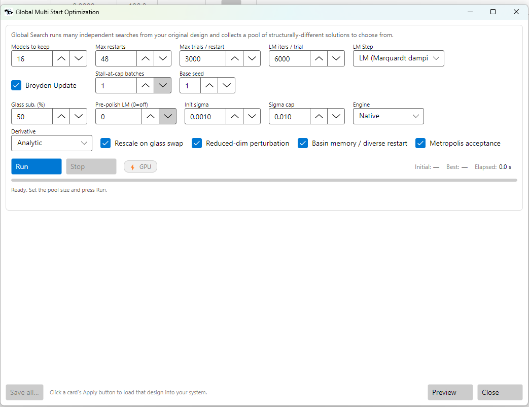
| Setting | Default | Meaning |
|---|---|---|
| Models | 16 | Target number of distinct designs to collect in the gallery. |
| Max Restarts | 48 | Upper bound on independent restarts (default 3× Models — restarts that land on an already-seen form are discarded, so you need several per kept model). |
| Trials / restart | 2000 | Multistart trial cap within each restart. |
| Base Seed | 1 | Restart i uses BaseSeed × 100000 + i. Run base seed 1, then 2, … for genuinely independent extra batches that never re-walk the same seeds. |
| Dedup tolerance | 0.02 | Two designs of the same form within this relative merit count as the same gallery entry. |
| Sigma, Glass Sub %, LM/Trial, Rescale on Glass Swap, … | Inherited from Multistart — each restart is a Multistart run. | |
| Reduced-dim perturbation, Basin memory / diverse restart, Metropolis acceptance | on | The three convergence levers, exposed here as their own checkboxes. Because each restart is a full Multistart run they behave exactly as in Multistart; on by default. |
| GPU pre-screen | off | Turned on globally in Editors ▸ Preferences ▸ GPU acceleration (Multistart GPU pre-screen (Beta)), not in this dialog. Every restart inherits the setting, so the gallery search gets the same basin-escape sieve. See GPU pre-screen. |
Every gallery entry is a complete, loadable .lhlt design. From the CLI the
pool is written to out=DIR (default global_search_results), one file per
rank named by rank, seed, merit, and glass set.
When to use it
Use Global Multi Start Optimization to survey the solution space of a specification — "what triplet forms reach this f/number and field, and with which glasses?" — rather than to drive a single design to its lowest merit. It costs more than one Multistart (it is many of them), but it surfaces alternative forms a best-only run hides. A good staged workflow: Global Multi Start Optimization to enumerate candidate forms → pick one → Local (or Basin Hopping) to refine it.
Global Evolutionary Optimization
Optimization → Global Evolutionary Optimization…
A population-based Differential-Evolution (DE) search that generates a pool of distinct starting designs from a poor — or even power-free — start (e.g. parallel plates), then polishes the best of them into a gallery. Where Multistart and Global Multi Start Optimization perturb one design at a time, DE evolves a whole population of candidates in parallel; and on an NVIDIA GPU the entire population is evaluated on-device every generation, so the search scales to tens of thousands of members. It is LensHH-LT's fastest route from "no design" to "a gallery of viable, polished starting forms."
The run has three stages:
- DE seed search. A population of trial designs is evolved for a number of generations. Each generation mutates and recombines members (DE/rand/1/bin) and keeps the better of trial vs. parent. Glass substitution is part of the search, so members explore both geometry and material.
- Focus + EFL conditioner (§8.5). After a member is formed, an optional fast solver refocuses it (a secant solve on a compensator thickness) and, when the merit has an EFL target, drives the effective focal length onto target (a Newton solve on a control curvature) — so the population stays near the spec instead of spending generations rediscovering focus. The surfaces it touches are user inputs (auto by default).
- Polish. The best N distinct seeds are polished — Multistart-LM by default (a full Multistart run per seed, like the standalone Multistart Optimization) or Local-LM — and shown as a gallery, best-merit-first. All pre-polish seeds are saved automatically, so the raw DE pool is never lost.
GPU is a flag, not a requirement: with a CUDA device the population is sized to fill the GPU automatically (≈6,000 designs on an RTX 4060, ≈34,000 on an H100); without one, the same search runs on the CPU at a population you set. The result is identical either way.
Settings
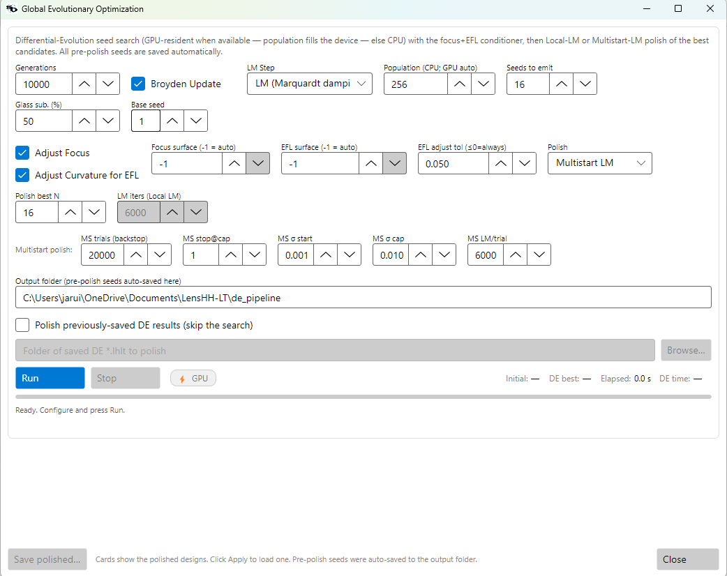
| Setting | Default | Meaning |
|---|---|---|
| GPU-resident DE | on if available | Turned on in Editors ▸ Preferences ▸ GPU acceleration (GPU-resident Differential Evolution), not in this dialog. On → the population runs on a CUDA device, sized to fill it. Off / no device → CPU at the Population you set. |
| Generations | 10000 | DE generations — the dominant cost knob. Reduce on CPU. |
| Population | GPU auto / 256 CPU | CPU population size. Ignored on GPU (auto-filled to device occupancy). |
| Seeds to emit | 16 | How many distinct seeds the DE keeps for polishing. |
| Glass sub. % | 50 | Probability a member draws a fresh glass per substitution-eligible surface, from the per-surface Glass Substitution Settings. |
| Base seed | 1 | RNG seed — the whole run reproduces from it: the DE search and the Multistart polish (each candidate's polish is seeded BaseSeed + rank). Same Base seed → identical results. |
| Focus+EFL conditioner | on | Master switch for the §8.5 per-member refocus + EFL solve. |
| Focus surface | auto | Surface whose thickness the focus solve adjusts. Auto = the airspace before the image plane. |
| EFL surface | auto | Surface whose curvature the EFL solve adjusts. Auto = the last powered surface. Only runs when the merit has an EFL target. |
| Adjust curvature for EFL | on | Off → refocus only, never touch curvature for EFL. |
| EFL adjust tol | 0.05 | Only solve EFL when the member is within this fraction of target (0.05 = ±5%); members further off are left for the merit to cull. ≤0 = always. |
| Polish | Multistart LM | How the best seeds are polished: Multistart LM (most thorough — a full Multistart run per seed), Local LM, or None (raw seeds). |
| Polish best N | 16 | How many of the best distinct seeds to polish. |
| LM iters | 4000 | LM iteration cap per candidate on the Local-LM path. |
| Output folder | …/de_pipeline | Pre-polish seeds are auto-saved here; the polished gallery can be saved too. |
| Polish previously-saved DE results | off | Skip the search and re-polish a folder of previously-saved seeds (see below). |
Live reporting
During a run the dialog reports, in order:
- DE phase — the running best merit, elapsed time, and average seconds per generation (so a long run's finish is predictable).
- DE complete — the best seed merit before any polish, and how many distinct seeds were found.
- Polish phase — which candidate is being polished ("Polishing 5 of 16"), that candidate's current best merit, and the best merit across the whole pool so far — whether the polish runs on the CPU or with the GPU pre-screen.
The same elapsed-time / seconds-per-generation figures and polish progress are
available from the CLI (optimize deseed) and the MCP (de_pipeline_status).
Polish a previously-saved DE result set
A DE search can take a while, and you don't have to repeat it to try a different
polish. Tick Polish previously-saved DE results, point the folder picker at a
saved seed folder (any folder of .lhlt files from a previous run — e.g. the
auto-saved seeds_pre_polish/), and the run skips the DE search and polishes
those designs with the current polish settings. Every file in the folder must
share the loaded design's structure (same surface count and merit operands); if
one doesn't, the run stops and names the offending file. From the CLI:
optimize deseed polish-folder=DIR; from the MCP: de_pipeline_start(..., polishFolder="DIR"); from the API: DePolishSavedSeeds(...).
When to use it
Reach for Global Evolutionary Optimization when you have no good starting design — a flat-plate or rough sketch — and want a spread of polished, viable forms quickly, especially on a GPU. It overlaps Basin Hopping (both can build a triplet from parallel plates) and Global Multi Start Optimization (both return a gallery), but it gets there by evolving a large population in parallel rather than perturbing one design — which is exactly what makes the GPU path so effective. A good staged workflow: Global Evolutionary Optimization to generate + polish candidate forms → pick one → Local (or Basin Hopping) to refine.
Case study: parallel plates → polished triplets (GPU)
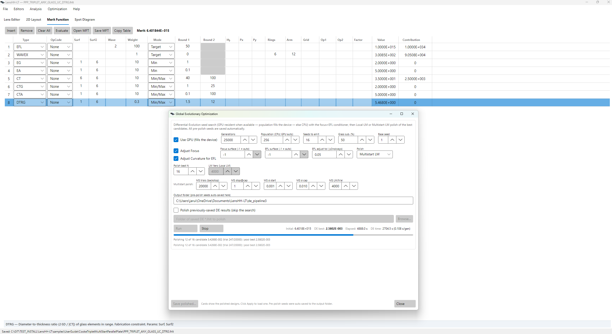
Sample:
samples/UserGuide/LensFilesForManual/PPP_TRIPLET_ANY_GLASS_UC.lhlt
— three flat plates, 50 mm EFL target, EPD 10, three fields, three wavelengths,
glass substitution on (CoreSet28). With Use GPU on, the population fills the
device automatically; the DE evolves it for the chosen number of generations, the
conditioner keeps every member near 50 mm EFL and in focus, and the best 16
distinct seeds are polished with Multistart-LM. The gallery comes back as a set
of structurally-distinct triplets, best-merit-first, with all pre-polish seeds
auto-saved alongside.
Basin Hopping (HJ + LM)
Optimization → Basin Hopping HJ+LM…
The deepest single-run explorer: one Basin Hopping run can travel far enough from the start to change topology (e.g. flat plates → Cooke triplet), where Multistart's small kicks cannot. (Global Multi Start Optimization explores along a different axis — it casts the widest net, collecting many distinct forms, rather than driving one design as far as possible.) Each hop runs:
- Random perturbation. Each continuous shape variable gets a
Gaussian kick of standard deviation
Sigma × variable_scale, pulling the design into a fresh starting point. Aperture semi-diameters and aspheric coefficients are not kicked — they are left for the LM to tune, so aperture/asphere noise doesn't disrupt the shape exploration. - Hooke-Jeeves pattern search. A derivative-free local search that works on the merit value alone. Steps along axes; expands the step on every successful direction; contracts only when no axis helps. Cheap and oblivious to local Jacobian smoothness — it's good at climbing out of shallow ridges that fool LM.
- LM refinement. Up to
LM/HopLevenberg-Marquardt iterations to land at the bottom of whatever basin HJ found. - Accept/reject. If the post-LM merit improves on the previous best, the hop is accepted and becomes the new starting point; otherwise the design reverts and the next hop perturbs from the best-so-far.
Optionally, every hop also swaps glasses on user-selected substitution-eligible surfaces, drawing from a filtered catalog. Glass swaps and continuous-variable hops cooperate: a swap that gets accepted often stays in the design while later hops fine-tune curvatures and thicknesses around it.
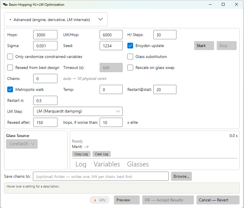
| Setting | Default | Meaning |
|---|---|---|
| Hops | 3000 | Outer-loop cap per chain. Reached less often than it looks: per-hop cost climbs as a design converges, so a long run can end on the clock rather than the cap. Lower it if you want the run to finish on its own. |
| LM / Hop | 6000 | Max LM iterations per hop. LM stops early on tolerance once a hop converges (~30 iterations for an easy basin), so this is generous headroom, not a fixed cost — a hop that is still improving is never cut off. Reduce only if you deliberately want shallow, cheap hops. |
| HJ Steps | 30 | Maximum Hooke-Jeeves steps per hop before handing off to LM. 30 is balanced; 0 disables HJ entirely. |
| Sigma | 0.001 | Starting value of the Gaussian-perturbation scale. Sigma is adapted automatically during the run (see below). 0.001 is sufficient even for severe starts; you rarely need to raise it. |
| Seed | 1234 | RNG seed. Change it to get a different random trajectory while keeping all other knobs identical — useful for confirming a result isn't a fluke. |
| Chains | 0 (auto) | Number of independent hopping chains run in parallel; the single best design across all of them is returned. 0 = automatic, one chain per physical CPU core. 1 = the classic single chain with the full live per-variable trace. Higher values fill the CPU and explore more basins at once — see Parallel chains. |
| Broyden Update | on | Same as Local LM. |
| LM Step | LM | Same meaning as for Local LM: PSD II / PSD III estimate per-variable curvature instead of using one damping value. Worth trying on designs with many variables, and where glass substitution matters. Selecting PSD turns Broyden Update off. |
| Only randomize constrained variables | off | Limit perturbation to bounded variables. Useful for surgical exploration when most variables are already where you want them. |
| Glass Substitution | off | Enable glass swaps. Pick the source from the Glass Source dropdown — filtered catalogs (small curated lists, cheap) or one of the loaded full catalogs (broad exploration, slower). |
| Glass Source | first filtered catalog | Pool used when Glass Substitution is on. Filtered catalogs in <install>/catalogs/Filtered/ are typically 30–100 glasses curated by status, manufacturer, refractive-index range, etc. See Glass Catalogs. |
| Reseed from best design / Timeout (s) | off / 600 | Per-chain watchdog. When on, a chain whose own best merit hasn't improved within this many seconds is reseeded from the best design found so far (a lone chain stops instead) — see Reseed from best design after no improvement. |
| Reseed after / if worse than | 150 hops / 10 × elite | Hand a chain another chain's design once it has gone this long without a best of its own and is this far out of contention — see Reseeding a chain that has fallen behind. 0 hops disables it. |
| Metropolis walk | on | Governs how a non-improving hop is handled. On (default): the chain may still accept a worse design as its next centre with probability exp(−ΔMerit/T), so it can step through a worse basin to reach a better one — thorough exploration. Off: greedy hopping — every non-improving hop is rejected and the chain restores to its best. Greedy converges quickly but can stick in the first basin. |
| Temp | 0 (autotune) | Metropolis temperature T in exp(−ΔMerit/T). 0 autotunes it to the mean of the first several uphill |ΔMerit| samples. Larger T accepts more worse moves (more exploration). Ignored when Metropolis walk is off. |
| Restart@stall | 20 | Full-range "long-jump" restart trigger (see Escaping a stalled search below). After this many consecutive hops with no new global best, the chain re-randomizes its shape variables across their whole range and continues from there. 0 disables it — a pure local walk that only reaches basins near the start. |
| Restart σ | 0.5 | Magnitude of that long-jump kick, in the same units as Multistart's Sigma Cap. 1.0 spans a variable's full bound half-range, like a Multistart trial; smaller values land on a traceable design more often. Only used when Restart@stall > 0. |
| Save chains to | (empty) | Folder to write every chain's final design (one .lhlt each) when the run finishes. Empty = keep only the global best in the workspace. See Saving every chain's design. |
Escaping a stalled search (full-range restarts)
New in 1.0.138. Basin Hopping's small per-hop kicks are ideal for refining a basin and for short hops to nearby ones, but on a hard design a chain can circle the same local minimum. When a chain goes a number of hops without a new best, it now performs a full-range restart: it returns to its best design, re-randomizes the shape variables (curvatures, thicknesses, glasses) across their whole range — the same magnitude a Multistart trial uses — and continues hopping from there. A restart that lands somewhere better is kept; otherwise the chain returns to its best and tries a fresh jump.
This gives each chain the global-restart reach that previously only Multistart had, layered on top of Basin Hopping's Hooke-Jeeves and LM refinement. In practice a Basin-Hopping run — especially with several parallel chains — now reaches the deep basins Multistart finds and polishes each one it visits, so it is competitive with (and often beats) Multistart on the same design instead of freezing at the first local minimum. The restart is on by default and needs no setup; since 1.0.146 you can tune when it fires (Restart@stall, in hops) and how far it jumps (Restart σ) from the dialog, or disable it entirely by setting Restart@stall to 0.
Reseeding a chain that has fallen behind (new in 1.0.152)
A full-range restart sends a chain somewhere new, but it is still a blind throw from where that chain already is. When several chains are running, one of them has usually already found something better — and a chain that is hopelessly behind is better off starting from that than from another random jump.
A chain is handed the best design found by another chain when both of these hold:
| Control | Default | Meaning |
|---|---|---|
| Reseed after | 150 hops | Hops with no new best of its own. |
| if worse than | 10 × elite | Its own best must be worse than this multiple of the best design any chain has found. |
Both conditions are required, and the second one is the important one. A chain that has gone quiet is not necessarily stuck: a Metropolis walk accepts uphill moves and routinely goes tens of hops between records while working perfectly well. Reseeding on the hop count alone would move nearly every chain onto the leader's design within the first few tens of hops — ten chains all exploring one basin is one chain with ten times the noise, and if that basin is a poor one, nothing is left to escape it. The merit factor is what keeps productive chains independent: a chain doing well by its own lights is never reseeded, however quiet it has been.
The chain holding the elite is never reseeded from itself, and the reseeded chain keeps its hop count — it is continuing, not starting over.
Set Reseed after to 0 to switch the mechanism off entirely.
Choosing the factor. If your chains typically finish within a factor of two of each other, a factor of 10 will never fire and the rescue does nothing. Read the per-chain merits in the Chains tab after a run and set the factor below the spread you actually see. Higher keeps more independent lineages; lower propagates a good design faster at the cost of diversity.
This is distinct from Restart@stall, which is the same chain restarting itself from its own best. That one keeps the chain in its own lineage and is what a single-chain run relies on; this one deliberately crosses lineages.
Parallel chains
A single hopping chain is sequential — one perturb-optimize step at a time — so it leaves most of your CPU idle. Set Chains above 1 (or leave it at 0 for one chain per physical core) to run several independent chains at once, each from its own random perturbation. They don't share state; the run simply returns the single best design found across all of them. Because each chain explores a different basin, a parallel run typically reaches a markedly better merit than one chain in the same per-chain hop budget — and it actually uses the cores you paid for.
While a parallel run is going, the Chains tab is the live view. Each row is one chain, showing its hops completed, running best merit, accepted/rejected counts, and a ◄ best marker on the chain currently holding the global best. The headline merit at the top of the dialog is the global best across all chains and only ever decreases; the log records each new global best as it's found. The Variables and Glasses tabs fill in at completion from the winning chain — while many chains are exploring different designs at once there is no single "current" design to track live.
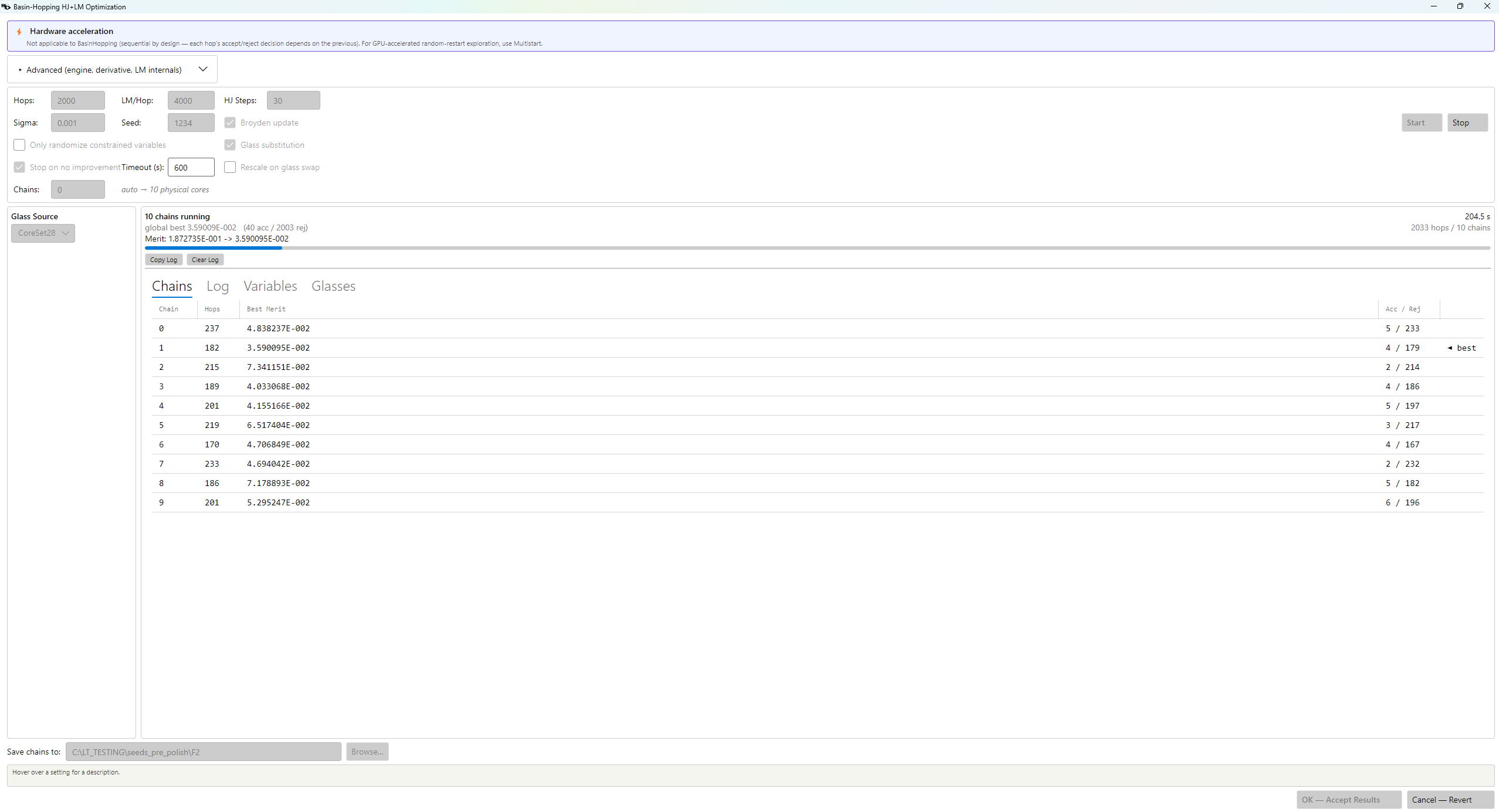
Chains = 1 is unchanged from earlier versions: one chain with the full live per-variable / per-glass trace in the Variables and Glasses tabs as it runs.
Physical vs. logical cores. Auto uses physical cores, leaving the hyperthread siblings free so the rest of the machine (and the app's own UI) stays responsive during a long run. On a dedicated machine you can set Chains to your logical core count for ~40 % more throughput at the cost of a busier system.
Reseed from best design after no improvement
Long runs often plateau well before they hit the Hops cap. This watchdog gives a chain that has gone quiet something better to do. Tick the box and set Timeout (s) to the idle window you're willing to wait.
The watchdog is per chain. Each chain runs its own timer, and the timer resets only when that chain's own best merit strictly improves — activity alone (rejected hops, equal-merit basins) does not reset it. The check happens between hops, so an in-progress hop always finishes and a long hop can overshoot the timeout by up to one hop's duration.
What happens when it fires depends on whether there is anything to borrow:
- With more than one chain, the quiet chain is reseeded from the best design found so far and keeps going. Unlike the hop-based trigger above, this does not apply the merit-factor test — if you have asked for a hard limit on idle time, it is taken at face value.
- With a single chain there is no sibling to borrow from, so the run ends — which is what this setting has always done, and what "no improvement for N seconds" can mean when a chain is on its own.
Changed in 1.0.152: with parallel chains this used to stop the chain. It now reseeds it, which is why the label reads "Reseed from best design" rather than "Stop on no improvement".
The timeout measures wall-clock time, not hop count, so its practical length
depends on how long each hop takes (LM/Hop, variable count, quadrature
density). Per-hop cost is not constant across a run: as a design converges the
inner LM has more work to do before it converges, so late hops can cost an order
of magnitude more than early ones. If a run is not reaching its Hops cap in
the time you expect, that is usually why — lower Hops rather than assume a
chain has stopped.
Saving every chain's design
By default a parallel run returns only the single global-best design,
loaded into the workspace. Set Save chains to (type a path or use
Browse…) to also persist every chain's final design as its own
.lhlt file in that folder when the run completes. Each chain explores a
different basin, so this captures the full spread of forms the run found —
useful starting points for a later split, asphere search, or a fresh
Multistart, not just the winner.
Files are written best-merit-first and named so they sort that way:
<base>_rank01_chain07_m3.59010E-002.lhlt   ← global best
<base>_rank02_chain03_m4.03307E-002.lhlt
<base>_rank03_chain09_m4.15517E-002.lhlt
…
rank01 is the global best; chainNN records which chain produced it;
mNNN is that design's merit. The shared merit-function definition is
embedded in each file. The same folder-save is available from the CLI,
MCP, and API so scripted runs persist their chains identically.
Sigma adapts during the run. The value you enter in the dialog is just the starting value; the optimizer grows or resets it between hops based on what's working:
- On reject: sigma is multiplied by 1.5. After a few consecutive rejections the per-hop kick has grown enough to push the design hard enough to cross into a different basin.
- On accept: sigma is reset to its starting value. A new minimum means the local region is fertile, so the next kick should be a small fine-tuning perturbation — not the inflated value left over from a recent rejection streak.
- At the 2.0 cap: if sigma's geometric growth would push it past 2.0 (a ~200 % relative kick), it is reset to the starting value instead of being parked at the cap. Without this, rejected hops near the cap fire huge perturbations that LM can't recover from in one hop's iteration budget — basin hopping gets stuck firing catastrophic kicks forever. The reset gives a clean small-kick restart and lets the optimizer climb back up via the 1.5× reject-growth ladder.
This adaptation is why setting Sigma very high rarely helps: the
optimizer escalates on its own when it needs to explore, and
collapses back to small steps the moment it lands in a productive
basin. The reset-on-accept also means you cannot reproduce a
previous run's trajectory by changing Sigma — only the starting
size of the first hop's kick is yours to set.
Aspheric coefficients are never randomly perturbed by Sigma in
Basin Hopping. Aspheric terms span many orders of magnitude
(A4 ≈ 10⁻⁶, A6 ≈ 10⁻⁹, A8 ≈ 10⁻¹²) and Basin Hopping skips them
unconditionally in the per-hop Gaussian kick. They are still
moved by Hooke-Jeeves pattern search and by the per-hop LM, just
not by the outer perturbation that drives basin-to-basin jumps.
If you want aspherics nudged across basins, run Multistart — its
per-order kick rule scales each coefficient by its natural
magnitude (1e-3 / y^(2(k+1)) for the k-th term).
Glass-substitution scope is determined by variables, not by an opt-in flag. Multistart and Basin Hopping use very different substitution mechanics:
- Multistart reads the per-surface table you populate in the
GUI's Glass Substitution dialog. Each surface has its own
Substitutecheckbox and its ownCatalogName— different surfaces can draw from different catalogs. See Glass Substitution During Optimization. - Basin Hopping doesn't use that table at all. The Glass Source dropdown in the BH dialog selects one filtered catalog and supplies every eligible glass element in the system. There is no per-surface flag.
A glass element is "eligible" only if it has at least one element-local variable — i.e., a variable the optimizer can move to compensate for an index swap:
| Variable on… | Lights up the element? |
|---|---|
| Front-face (S_i) curvature | Yes |
| Front-face thickness (= glass thickness) | Yes |
| Front-face conic / aspheric coefficient | Yes |
| Back-face (S_(i+1)) curvature | Yes |
| Back-face conic / aspheric coefficient | Yes |
| Back-face thickness (= air gap after the element) | No |
The last row is the subtle one: a variable air gap after a glass element lets the optimizer move the next element axially, but can't reshape this glass — so swapping its index would land in a basin LM has no degrees of freedom to climb out of. Such elements are quietly skipped, with a log line at run start:
Glass source: S1_GLASS (28 glasses)
Substitution-eligible elements: 2 of 3 (1 fixed glass has no active variable — not eligible)
If you intended an element to participate but it's reported skipped, mark a curvature, conic, or glass-thickness variable on one of its faces.
Case study: Basin Hopping on the Cooke triplet
Basin Hopping runs the same HJ+LM engine as Multistart, but it
chains its hops: each hop perturbs the current best and accepts or
rejects it by a Metropolis rule, so it explores by walking rather than
restarting cold. On the same triplet
(samples/UserGuide/LensFilesForManual/CookeTriplet_UC.lhlt, merit
0.0794) it reaches deeper minima than Multistart — and it is far
more robust from a bad starting point.
Settings are the defaults except Glass Source = CoreSet28 and Chains = 0 (auto), which on this machine launched 10 parallel chains, one per physical core. Each chain explores its own basin; the header merit is the single global best across all ten and only ever decreases.
Fixed glass
With glasses held fixed, Basin Hopping reaches the very same basin Multistart found — independent confirmation that 0.0429 is the real continuous-variable optimum for this triplet:
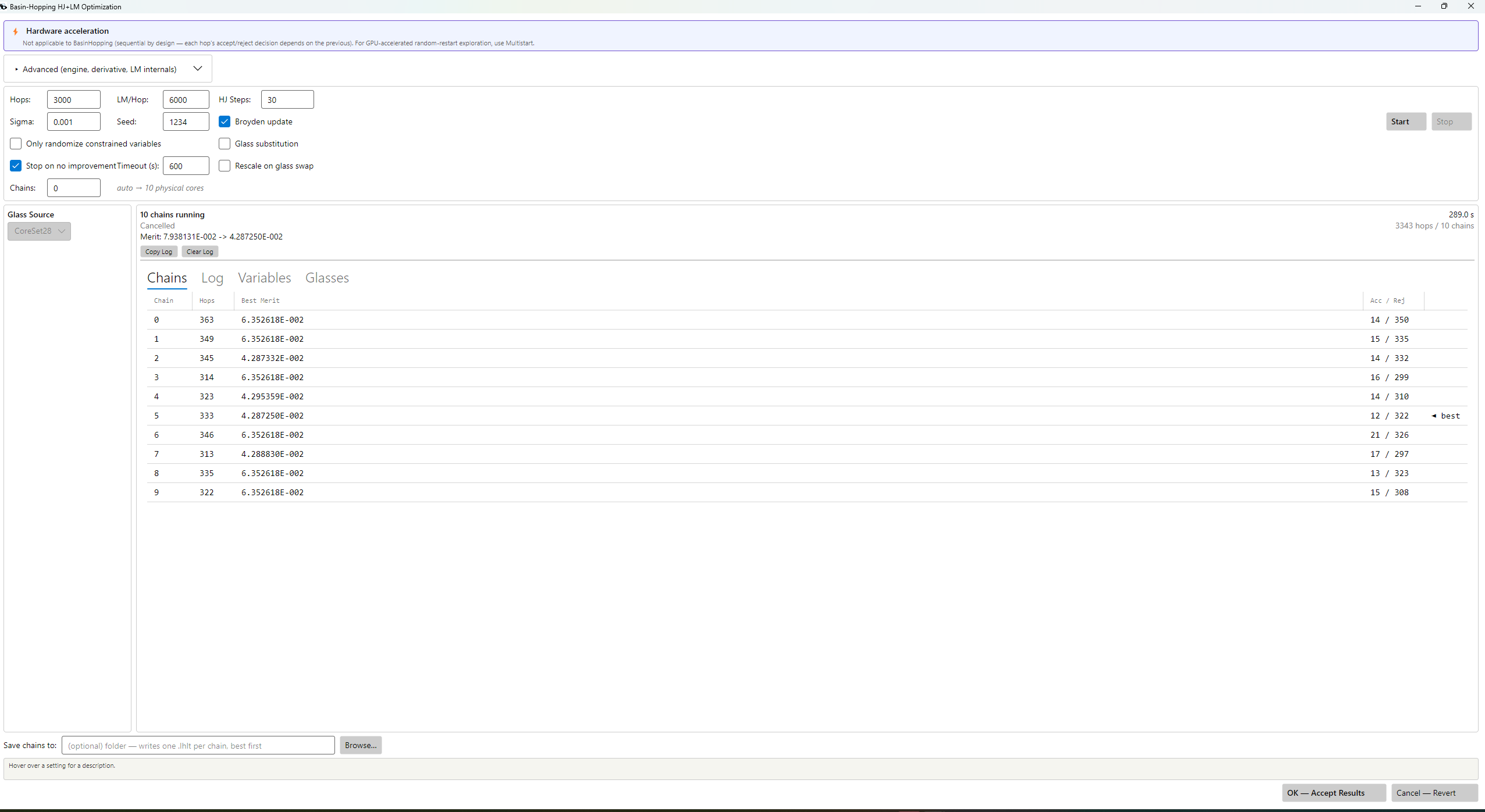
Result: 0.0794 → 0.0429 (289 s, 10 chains). Several chains reached 0.0429 while the rest settled near 0.063 — the spread across chains is the method telling you which basin is genuinely deepest.
Glass substitution on
Allowing substitution from CoreSet28, Basin Hopping digs well past Multistart's 0.0276:
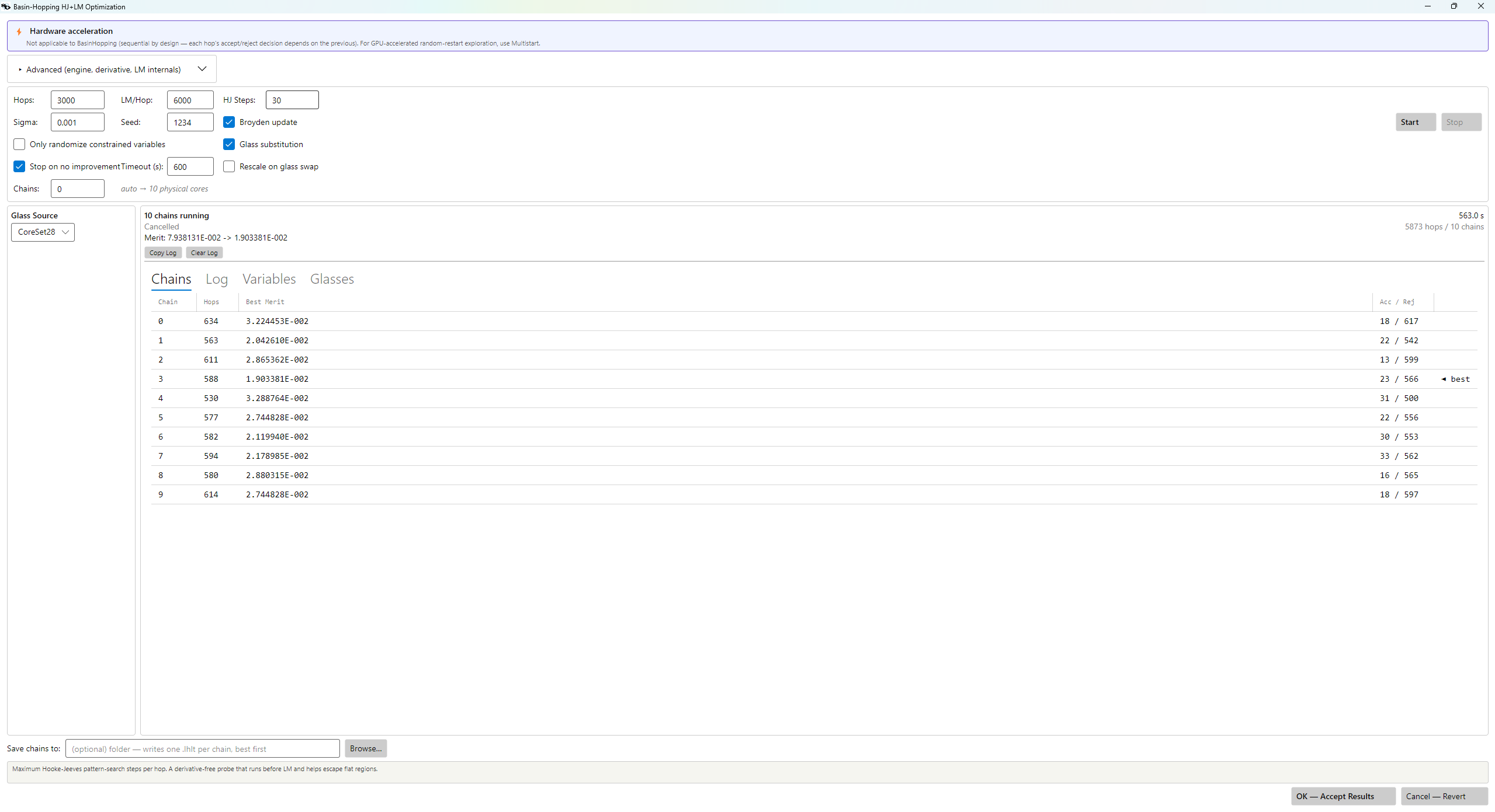
Result: 0.0794 → 0.0190 (563 s) — the deepest minimum any method reached on this design.
| After — wavefront | After — FFT MTF |
|---|---|
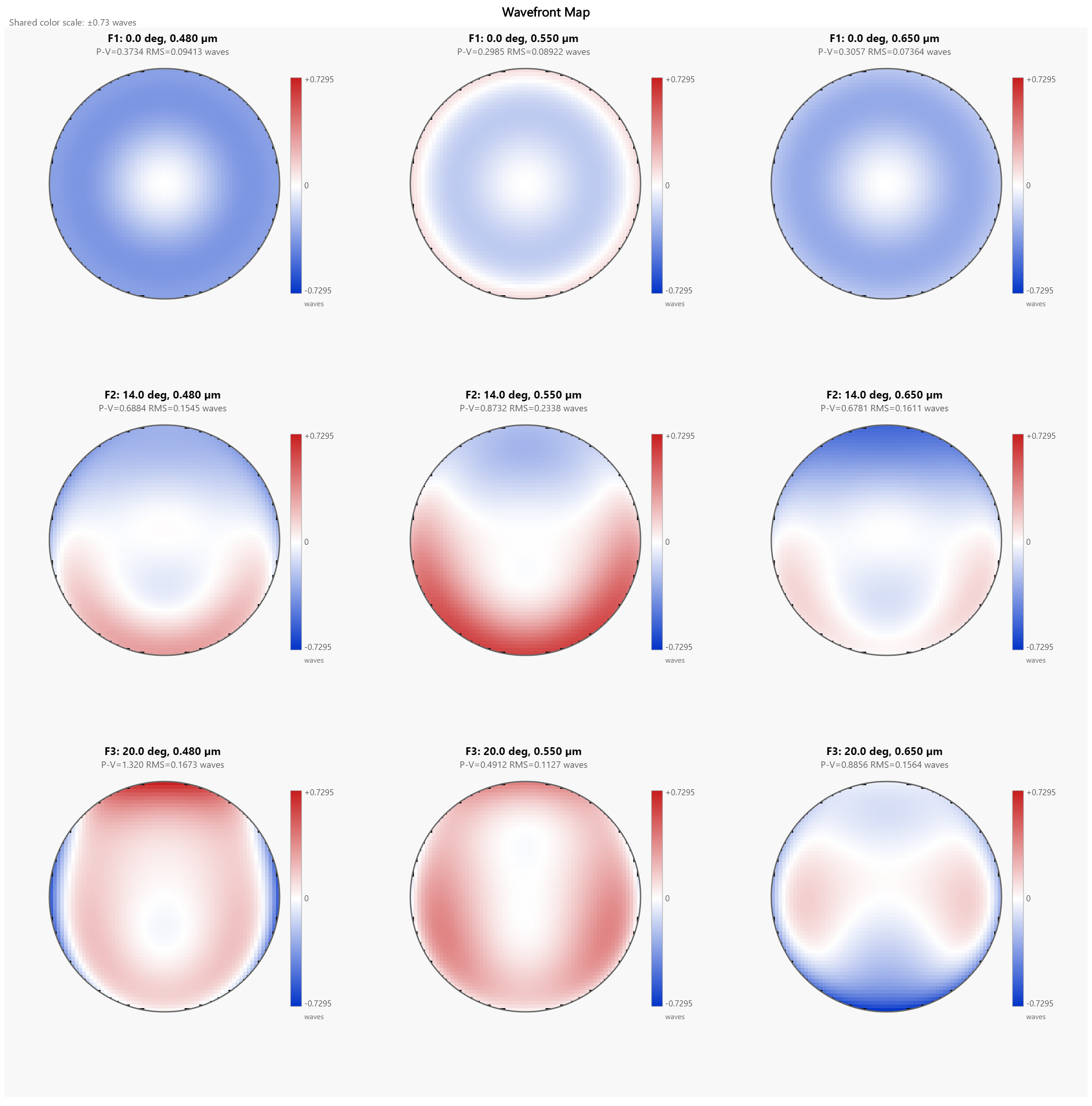 |
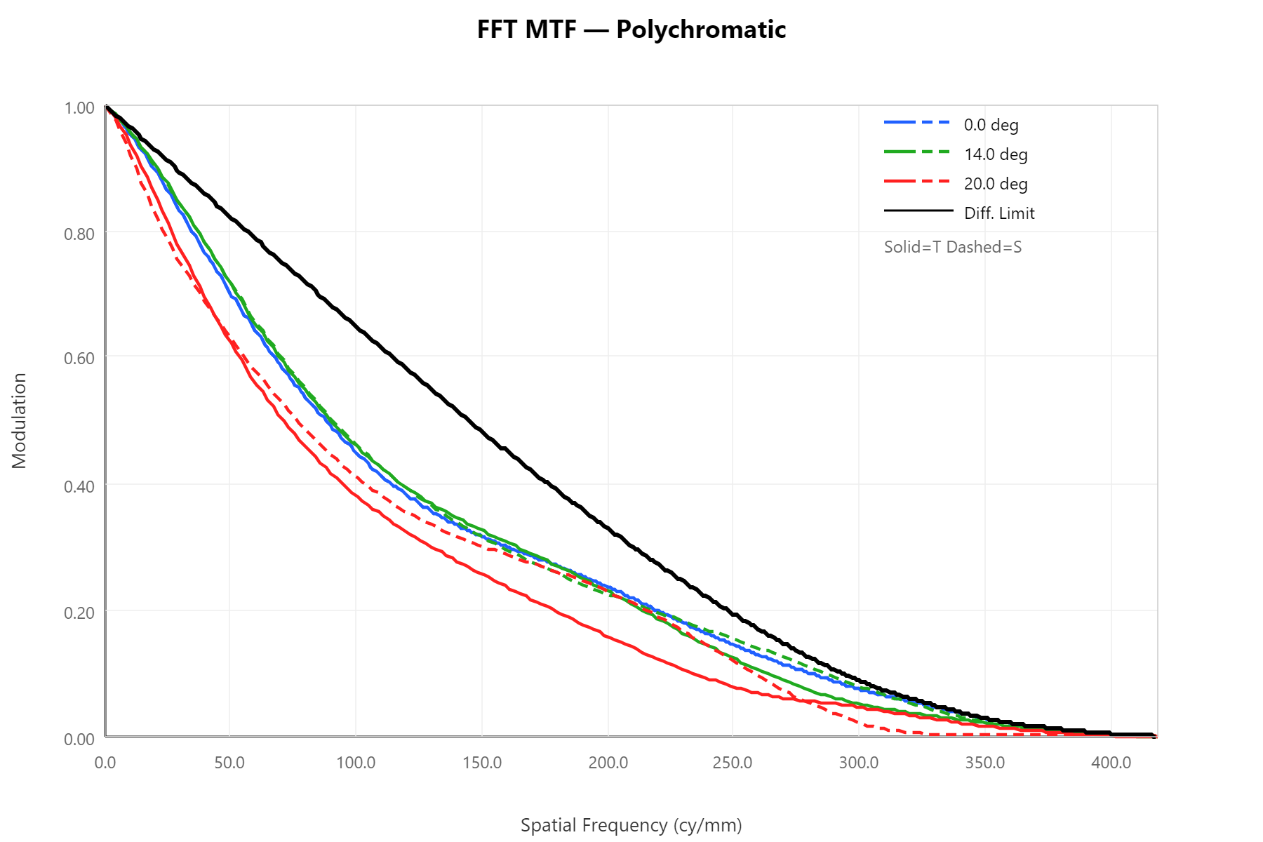 |
From a bare parallel plate — and why Basin Hopping is more reliable
The demanding test: hand Basin Hopping the same three flat plates Multistart got — every radius infinity, merit 8.0 × 10¹⁴ — and let it rebuild the lens from nothing.
| Before — three flat plates | After — Basin-Hopping triplet |
|---|---|
|
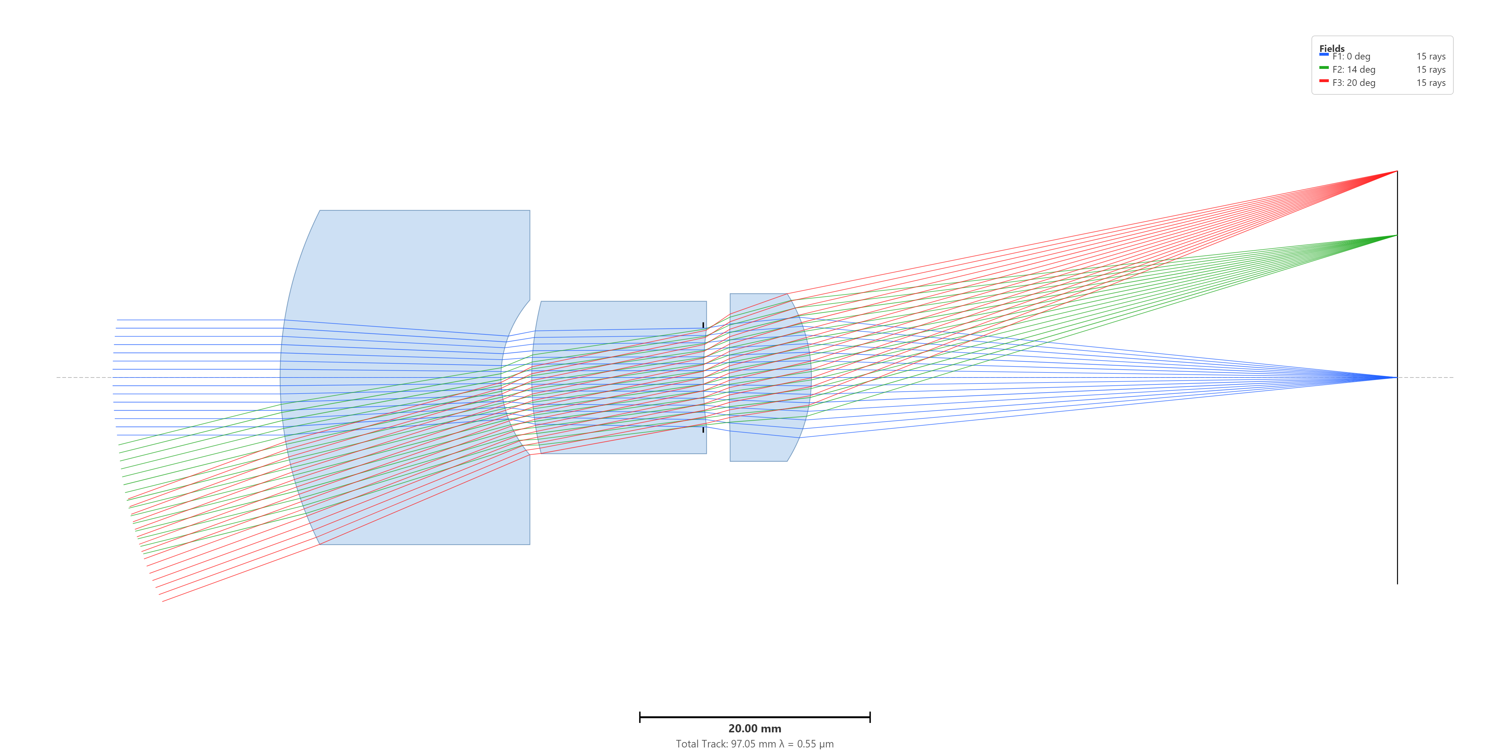 |
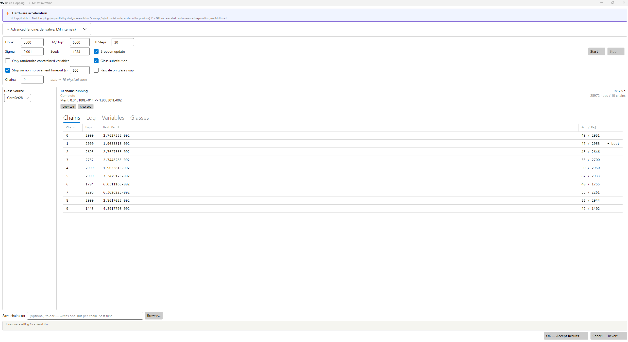
Result: 8.0 × 10¹⁴ → 0.0190 (1837 s, 25 972 hops across 10 chains). That is the same 0.0190 Basin Hopping reached from the finished triplet — the optimum is starting-point-independent; it simply took longer to get there from nothing. The header also shows the Phase-1 LM leaving the plate untouched at 8.0 × 10¹⁴ (a zero-curvature surface has no gradient), so every bit of progress came from the hops. The converged design is a recognizable Cooke triplet — positive front, negative middle around the stop, positive rear — built from glasses the substitution step chose, not any the user specified:
| Spot | FFT MTF |
|---|---|
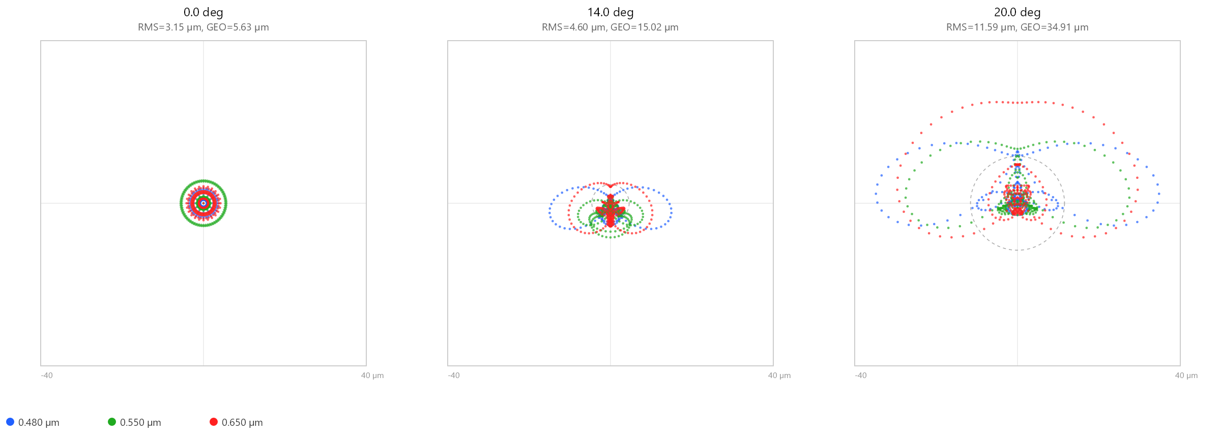 |
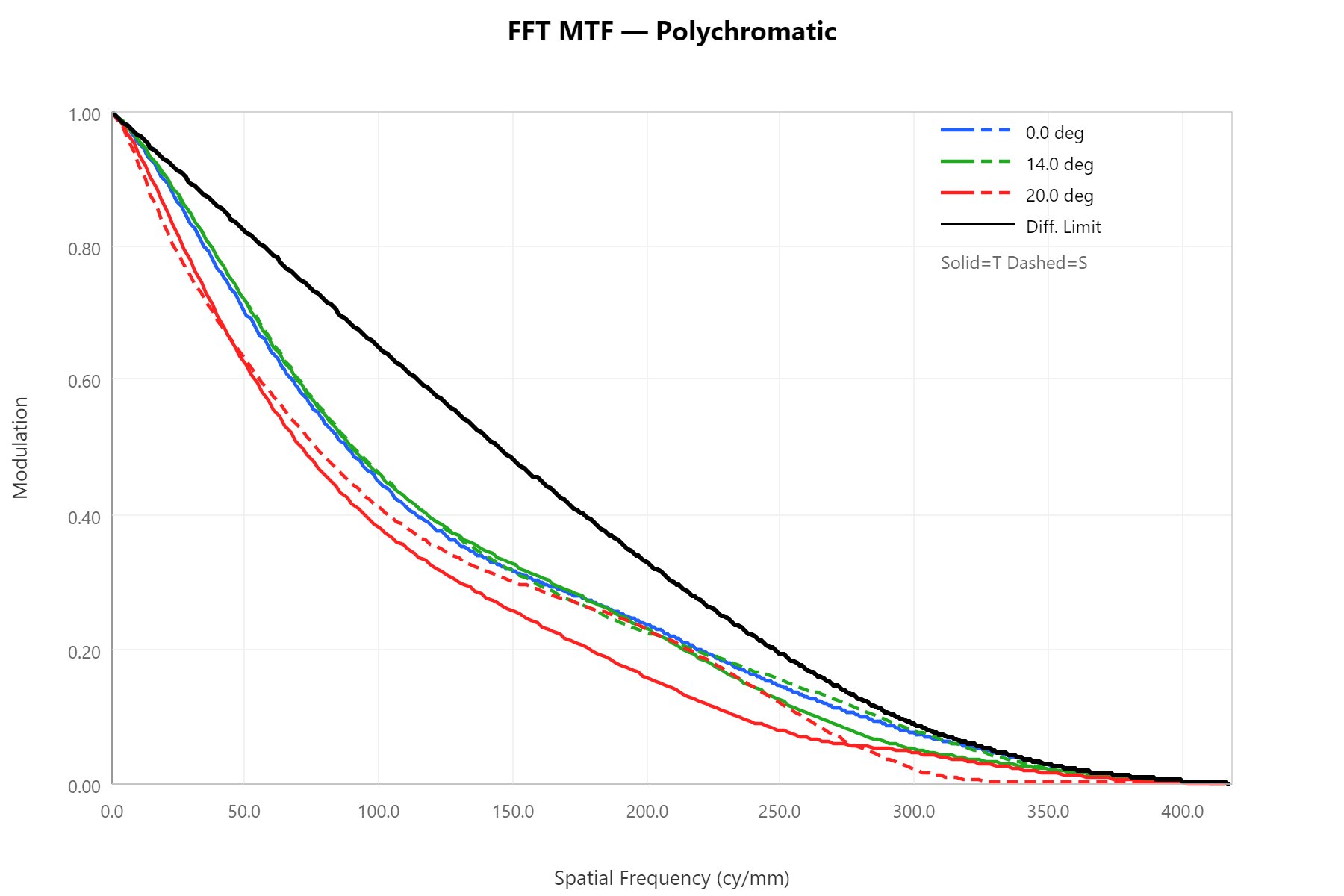 |
Basin Hopping vs Multistart from the plate. From the identical flat-plate start, the two methods diverge:
| Method | Result from the plate | Time |
|---|---|---|
| Multistart, glass sub | 0.0287 | 95 s |
| Basin Hopping, glass sub | 0.0190 | 1837 s |
Multistart's independent restarts each land in whatever basin they happen to hit, and it keeps the best — here that plateaus near ~0.028. Basin Hopping's chained hops, with the Hooke-Jeeves pattern search running before each LM, walk out of shallow basins toward the deepest one. So Basin Hopping is slower but more reliable when the start is far from any good design; Multistart is faster and, with the GPU pre-screen, scales to far more restarts. After either, the standard finish is a Local LM pass for the last fraction of a percent.
Reading the log
A parallel run (Chains > 1) is too noisy to print every hop from every chain, so the log records only new global bests — the moments when some chain beats the best merit any chain had reached so far:
new global best  6.086659E-002   (hop 369)
new global best  5.276065E-002   (hop 1258)
new global best  2.979231E-002   (hop 1283)
The hop number is a cumulative counter across all chains, so it climbs faster than any single chain's own hop count. The header keeps the running totals — global best merit, and cumulative accepted / rejected / glass-swap counts — and the Chains tab shows each chain's own progress with a ◄ best marker on whichever chain currently holds the global best.
With Chains = 1 the log is the classic per-hop trace instead:
Hop  14 [ACC] merit=4.87551E-002  best=4.87551E-002  glass-swaps=1
Hop  15 [rej] merit=5.37427E-002  best=4.87551E-002
[ACC] means the post-LM merit beat the previous best; glass-swaps=N
is how many glass surfaces were re-randomized for that hop. When a hop's
merit is dramatically larger than best (10⁴–10⁵), the perturbation
pushed the design into a non-tracing or broken state that LM couldn't
recover from — those hops simply get rejected.
Watch for two patterns:
- Quick early plunge, long tail. Like the case study: most of the gain in the first fraction of the run, then slow refinement. Normal.
- Long flat plateau. Global best unchanged for a long stretch. Either you're at the best form for the chosen topology and glass pool, or you need a larger Sigma, more variables, or a broader substitution catalog — that's what the Reseed from best design watchdog is for.
Global Basin Hopping (HJ + LM)
Optimization → Global Basin Hopping HJ+LM…
Global Basin Hopping is the cooperative, run-until-you-say-stop version of parallel Basin Hopping. Plain parallel basin hopping launches one chain per core, runs each to completion once, and returns the best; the global version never stops a chain — when a chain stalls it restarts from the best basin any other chain has found and keeps digging, for as long as you give it. Where Global Multi Start casts the widest net (a gallery of distinct forms), Global Basin Hopping drills the deepest single answer: all the chains pool their best basin and pile effort into it.
The loop, per chain:
- Run a basin-hopping episode (the same hop = perturb → Hooke-Jeeves → LM → accept/reject loop described above) with your settings.
- The episode ends when either the per-chain no-improvement watchdog fires (best merit hasn't improved within the timeout) or the chain reaches its Hops cap.
- The chain then restarts, seeded with a clone of the best design found so far by all the other chains (excluding its own), with its random seed advanced so it doesn't retrace — and goes back to step 1.
- This continues until the global time limit elapses or you press Stop.
This is why the watchdog is mandatory here (you can only edit its timeout, not turn it off): the restart-from-elite migration is the entire mechanism, and a chain has to be allowed to stall in order to jump to a better basin.
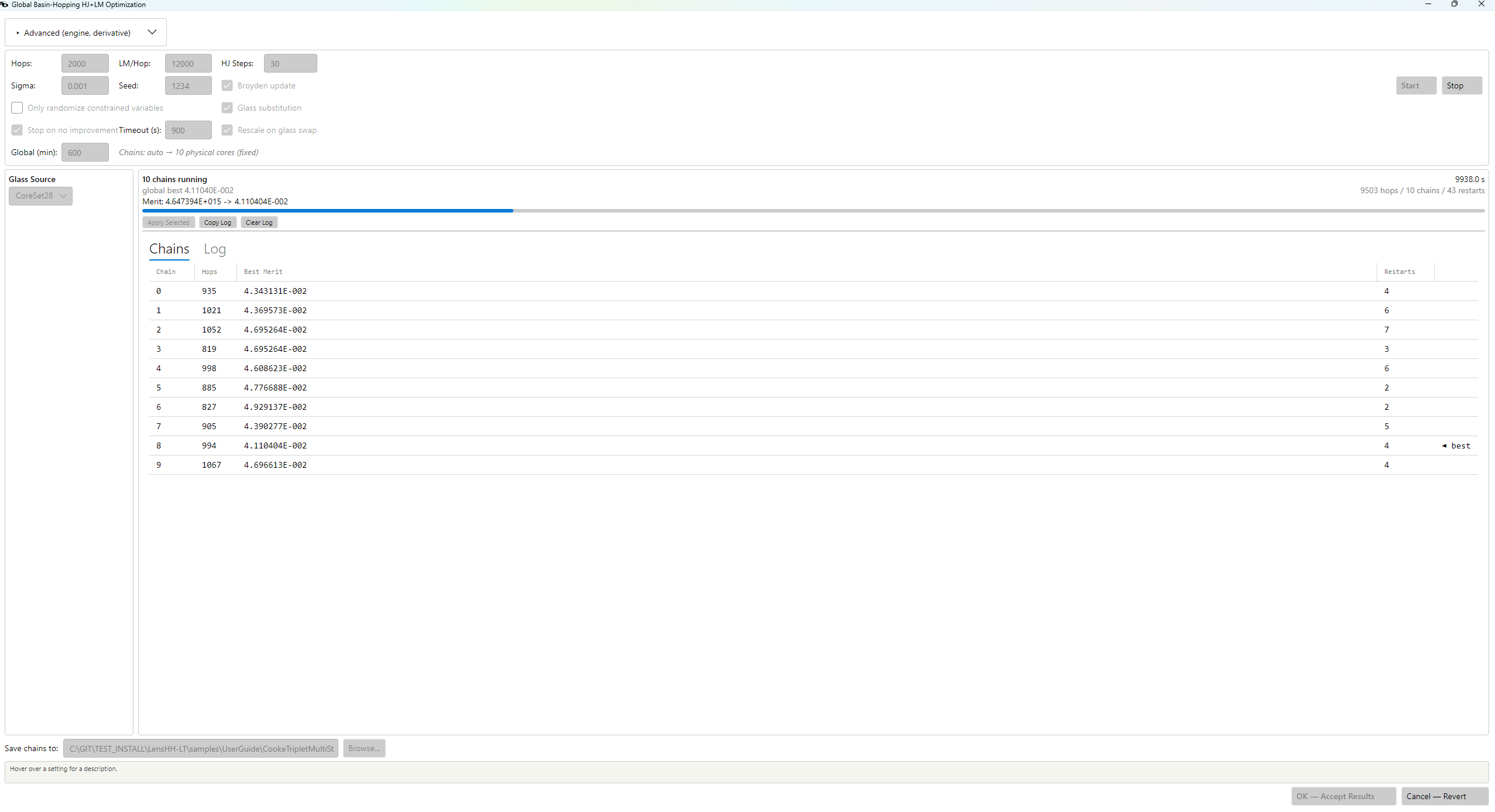
Settings
The per-chain HJ-LM knobs are the same as Basin Hopping — Hops, LM/Hop, HJ Steps, Sigma, Seed, Broyden update, Glass substitution, Rescale on glass swap, Only-randomize-constrained, the Glass Source, the Metropolis walk (with its Temp), and the full-range restart (Restart@stall, Restart σ) — and behave identically inside each episode. The differences are the three controls that govern the global loop:
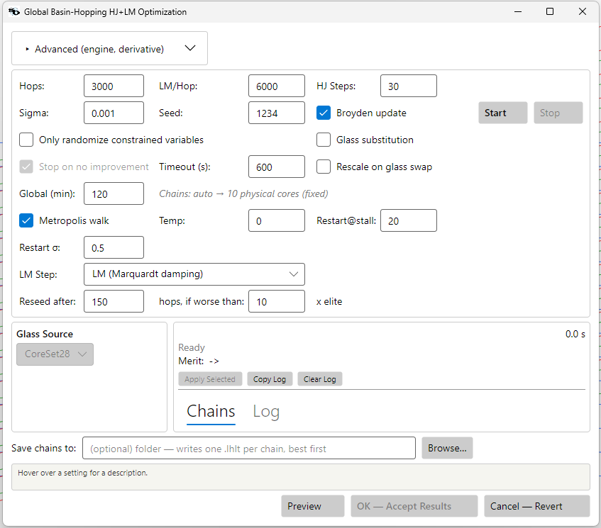
| Setting | Default | Meaning |
|---|---|---|
| Chains | auto (physical cores) | Fixed — not editable. One chain per physical core; shown read-only as "auto → N physical cores". |
| Stop on no improvement / Timeout (s) | on / 600 | Always on. A chain restarts (from the elite of the other chains) when its best merit hasn't improved within this many seconds. Only the timeout is editable. |
| Global (min) | 120 | Total wall-clock budget. The whole run stops when this elapses (or you press Stop). 0 = run until you stop it. |
Hops is now the episode cap rather than the run length — set it high (the
default 2000 rarely caps an episode before the watchdog does) unless you
specifically want short, frequent restarts.
Reading the dialog
- Header (e.g. "9503 hops / 10 chains / 43 restarts") — totals across the whole run: every hop summed over all chains, and how many times chains have reseeded from the elite.
- Chains tab — one row per chain:
- Hops is that chain's cumulative total; it does not reset on restart (so the per-chain Hops sum equals the header's total).
- Best Merit is the chain's best-ever design.
- Restarts counts how many times that chain has reseeded from the others.
- ◄ best marks the chain currently holding the global best.
A healthy run shows the per-chain Best Merit values converging — that's the elites propagating — while Restarts climbs as stalled chains keep jumping to the shared best basin.
Finishing
When the run ends, the Chains tab becomes a gallery of each chain's best
design (sorted best-first, the global best pre-selected). The global best is
already applied to your system; to take a different chain instead, select its row
and click Apply Selected. Set Save chains to to write every chain's best
design as its own .lhlt (best-merit first) — feed those into a later
Split Element, asphere search, or a fresh Multistart.
Global Basin Hopping is available everywhere the other optimizers are: the GUI
dialog above, the CLI (optimize global-basin … timeout= globalmin= savechains=),
the MCP tool global_basin_hopping_start (non-blocking — poll optimize_status),
and the .NET API (IOptimization.GlobalBasinHopping).
Split Element
Optimization → Split Element
Adds a degree of freedom to a converged design by splitting a glass element into two thinner elements with a small air gap between them. The motivation is the same one that turned the classical Cooke triplet into a four-element Tessar: at some point the existing surface count runs out of correction power and the only path forward is more surfaces. Multistart and Basin Hopping can move the design around in the space it has; Split Element grows the space.
A run does five things in order:
- Pick an element. Each element gets an aberration score
from the sum of
|S1| + |S2| + |S3|(spherical + coma + astigmatism Seidel coefficients) across its two surfaces; the highest scorer is the candidate. The log lineSelected: surface 5 (N-PSK53A), aberration score: 0.27reports the chosen element by its front surface and material. - Insert the new surface. The element is split into a
front-glass + air-gap + back-glass triple, sized so the
geometry initially preserves the parent's optical effect.
Merit jumps temporarily because the merit function now has
two more thickness operands and the new airspace adds an
EArow. - Pre-glass Multistart (with the original glass on both halves of the split). Continuous variables only. Walks the merit down to whatever the new geometry can do without changing materials.
- Glass trials. Enumerates pairs of glasses from the
selected filtered catalog and runs a short LM on each pair.
The capped count (
Glass Trials) sets the budget; the actual number can be smaller after the catalog filters out incompatible pairs (the run below tried 202 of 300). - Post-glass Multistart (with the best pair from step 4) refines around the new material choice.
Both Multistart phases auto-advance after a configurable idle
window (Skip phase if no improvement for (s) — default 600 s)
so a stuck phase doesn't block the run.
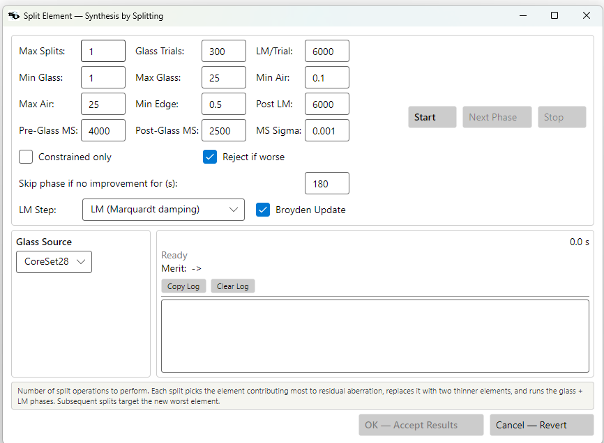
| Setting | Default | Meaning |
|---|---|---|
| Max Splits | 1 | Number of split passes. Each pass picks the highest-aberration surface from the current state and splits it. |
| Glass Trials | 300 | Cap on glass-pair combinations tried in the glass-trial phase. Actual count may be lower after catalog-pair filtering. |
| LM/Trial | 4000 | Per-trial LM iterations during glass trials. |
| Pre-Glass MS | 4000 | Multistart trials before glass swaps. |
| Post-Glass MS | 2500 | Multistart trials after the best glass pair is locked in. |
| Post LM | 4000 | Final LM iteration cap after both Multistart phases. |
| MS Sigma | 0.001 | Init Sigma for both Multistart phases — the same grow-on-rejection schedule as the standalone Multistart. |
| Min Glass / Max Glass | 1 / 25 mm | Centre-thickness bounds enforced on the split's glass halves. |
| Min Air / Max Air | 0.1 / 25 mm | Bounds on the new air gap between the split halves. |
| Min Edge | 0.5 mm | Minimum edge thickness on the split element. |
| Skip phase if no improvement for (s) | 600 | Idle window before a Multistart phase auto-advances. |
| Constrained only | off | Per-Multistart-phase setting; restricts perturbation to bounded variables. |
| Reject if worse | on | If the post-pass merit is worse than the pre-split merit, the original geometry is restored. The merit usually improves substantially, but this is the safety net. |
| Glass Source | first filtered catalog | Filtered catalog supplying glass-pair candidates. Cherry-picked or criteria-built — see Glass Catalogs. |
Case study: post-Multistart Cooke triplet → split element
Sample files: samples/UserGuide/CookeTripletSplit/. The starting state
is a Cooke triplet that was first synthesized from three parallel
plates (finite conjugate, 500 mm working distance) by Multistart
with glass substitution. By the time Split Element runs, the
design is already at merit 2.19 × 10⁻³ and Local LM finds no
further improvement.
| Before — converged Cooke triplet | After — split rear element |
|---|---|
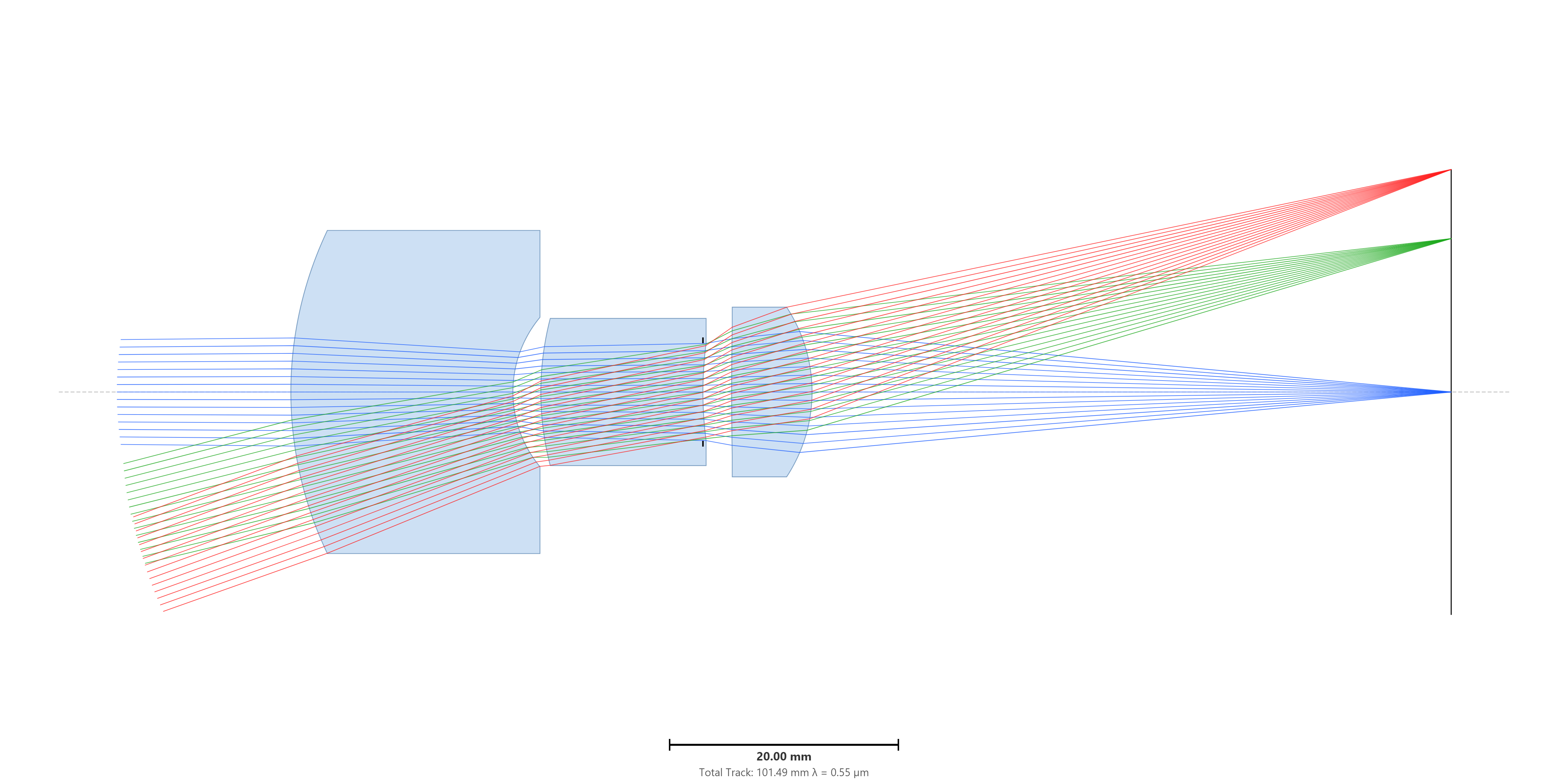 |
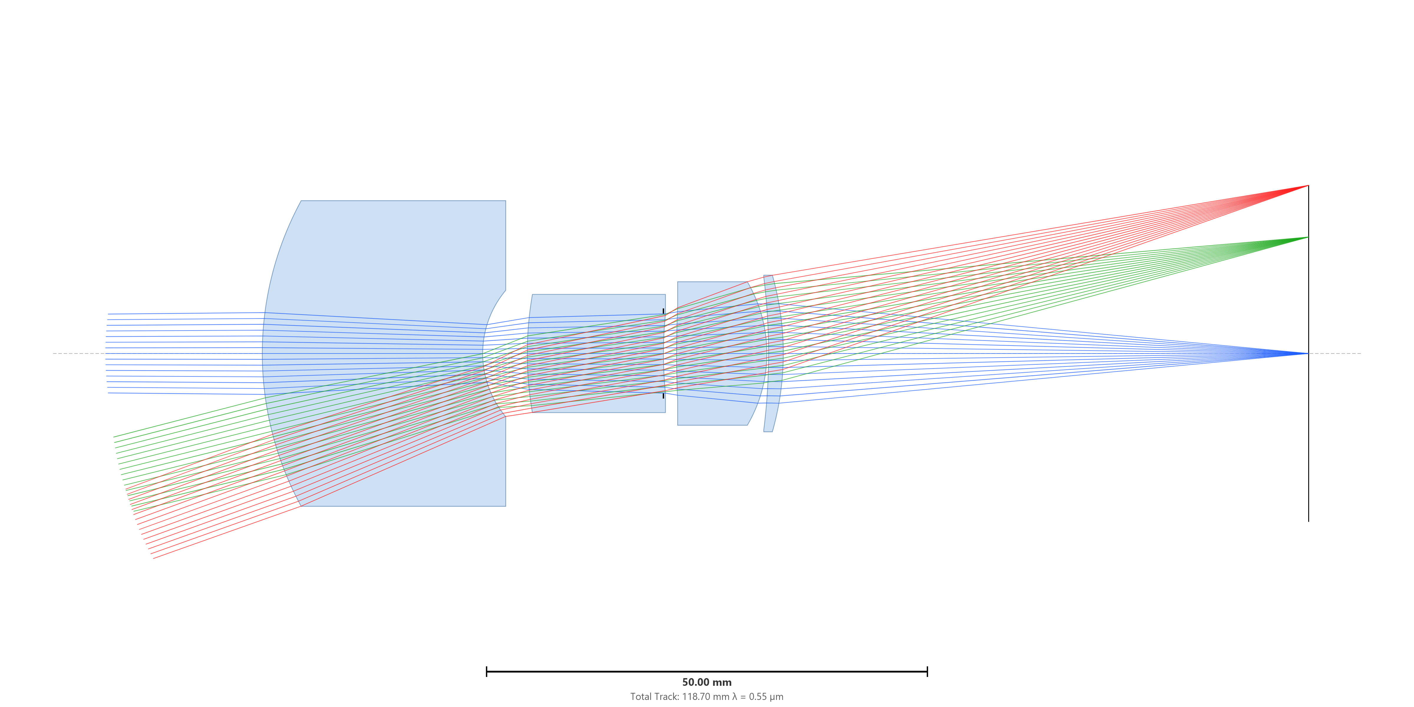 |
Settings: defaults except Glass Source = CoreSet28. The dialog
on completion:
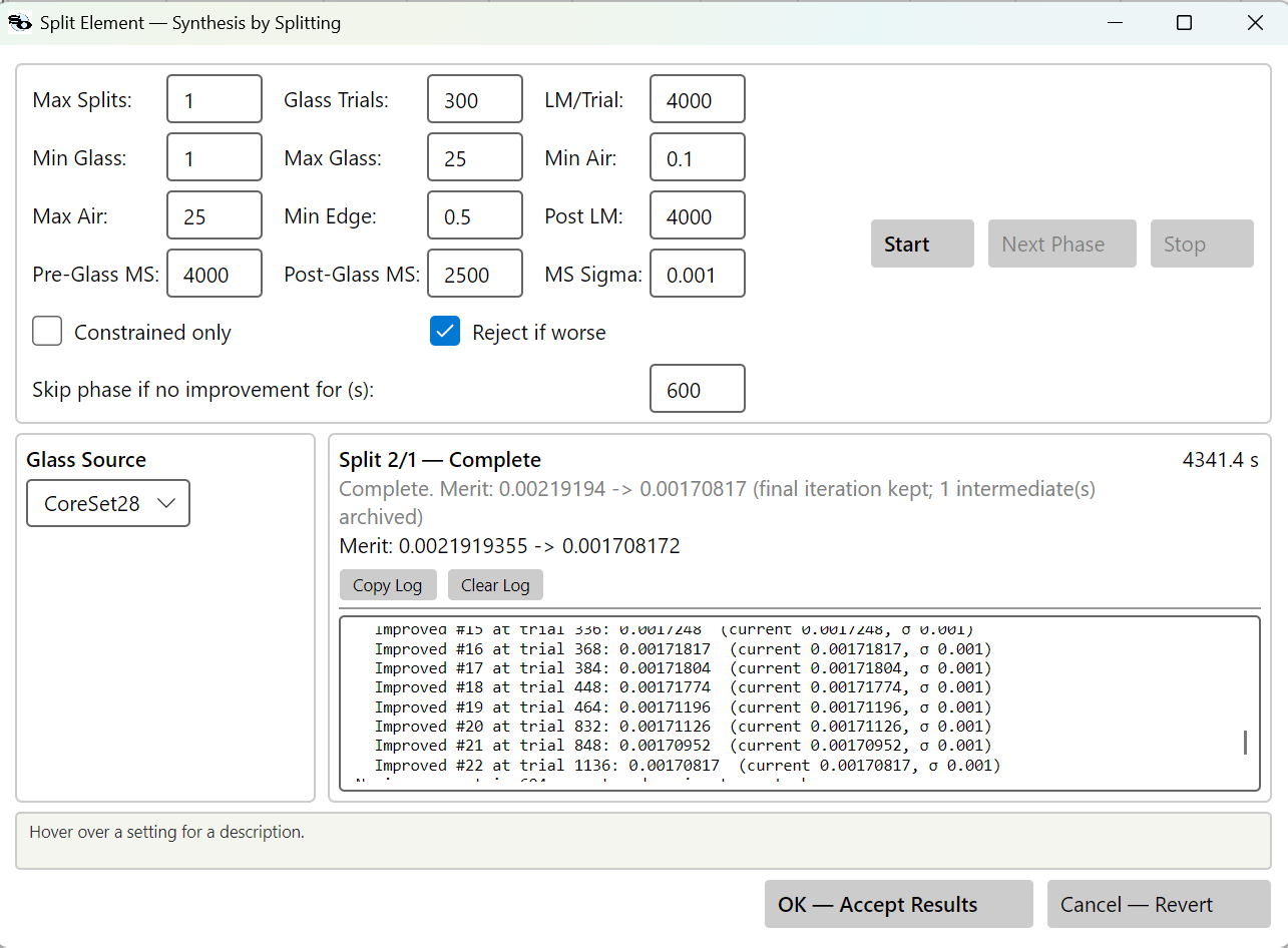
The trajectory from the log:
| Phase | Merit | Note |
|---|---|---|
| Start | 0.00219 | Converged Cooke triplet input. |
| Surface picked | — | Surface 5 (N-PSK53A), aberration score 0.27. |
| After insertion | 41.4 | Merit spikes — new operands and a 3-into-3 element split with the original glass on both halves. |
| Pre-glass MS, trial 16 | 0.0131 | Continuous variables alone recover most of the geometry. |
| Pre-glass MS, trial 704 | 0.00193 | 39 improvements; auto-advances after 610 s idle. |
| Glass trials, trial 124 | 0.00188 | Best pair: N-FK58 + N-LAK10. Tried 202 of 300 generated combinations. |
| Post-glass MS, trial 1136 | 0.00171 | 22 further improvements; auto-advances after 604 s idle. |
| Final | 0.00171 | Total wall-clock 4341 s (≈ 72 min). |
Net: merit 0.00219 → 0.00171 (~22 % reduction). Total track
grew from 101.5 mm to 118.7 mm. The headline gain is modest
relative to what Multistart and Basin Hopping had already done,
but it's gain you cannot get without adding the surface — the
input was the floor of its own basin.
| Spot before | Spot after |
|---|---|
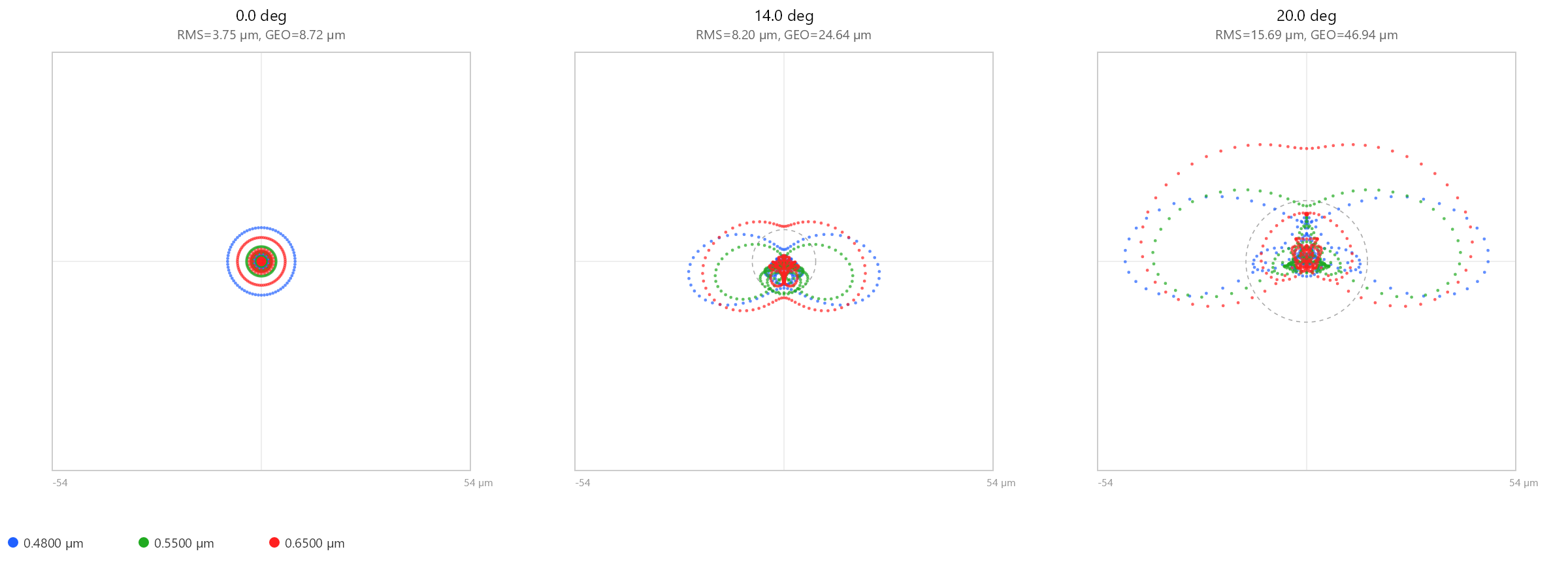 |
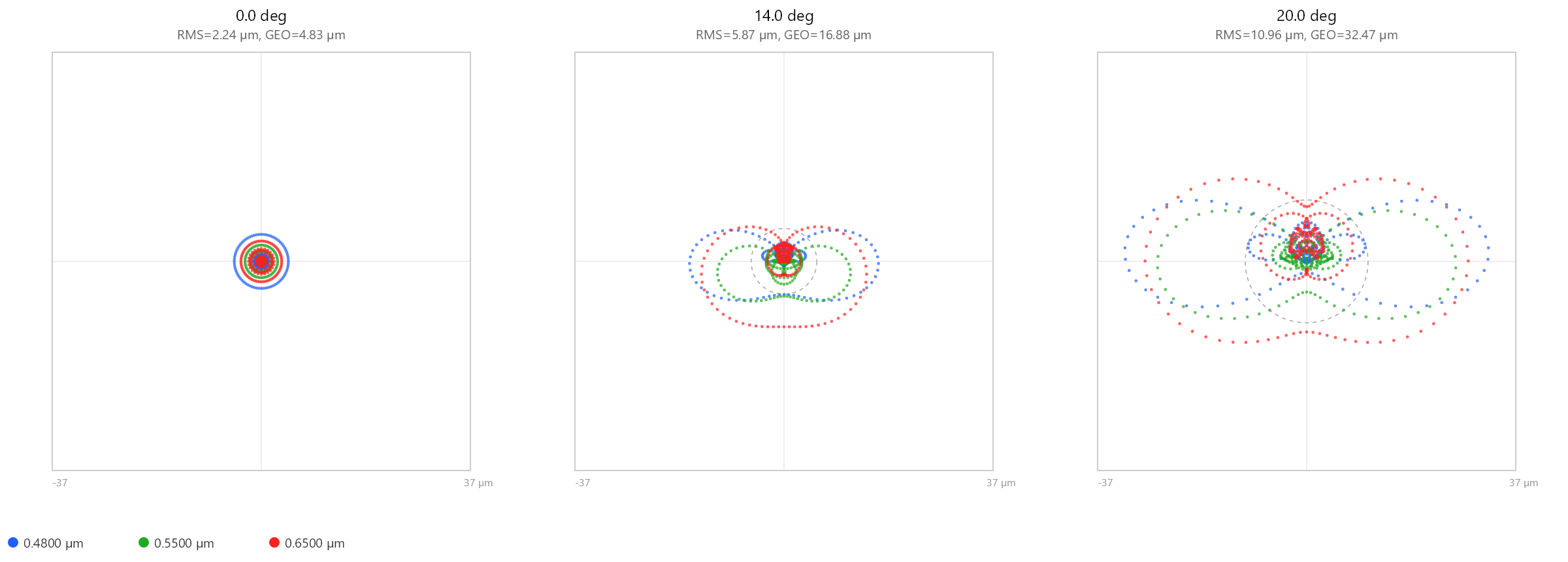 |
| FFT MTF before | FFT MTF after |
|---|---|
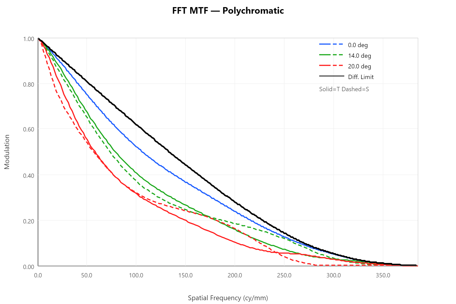 |
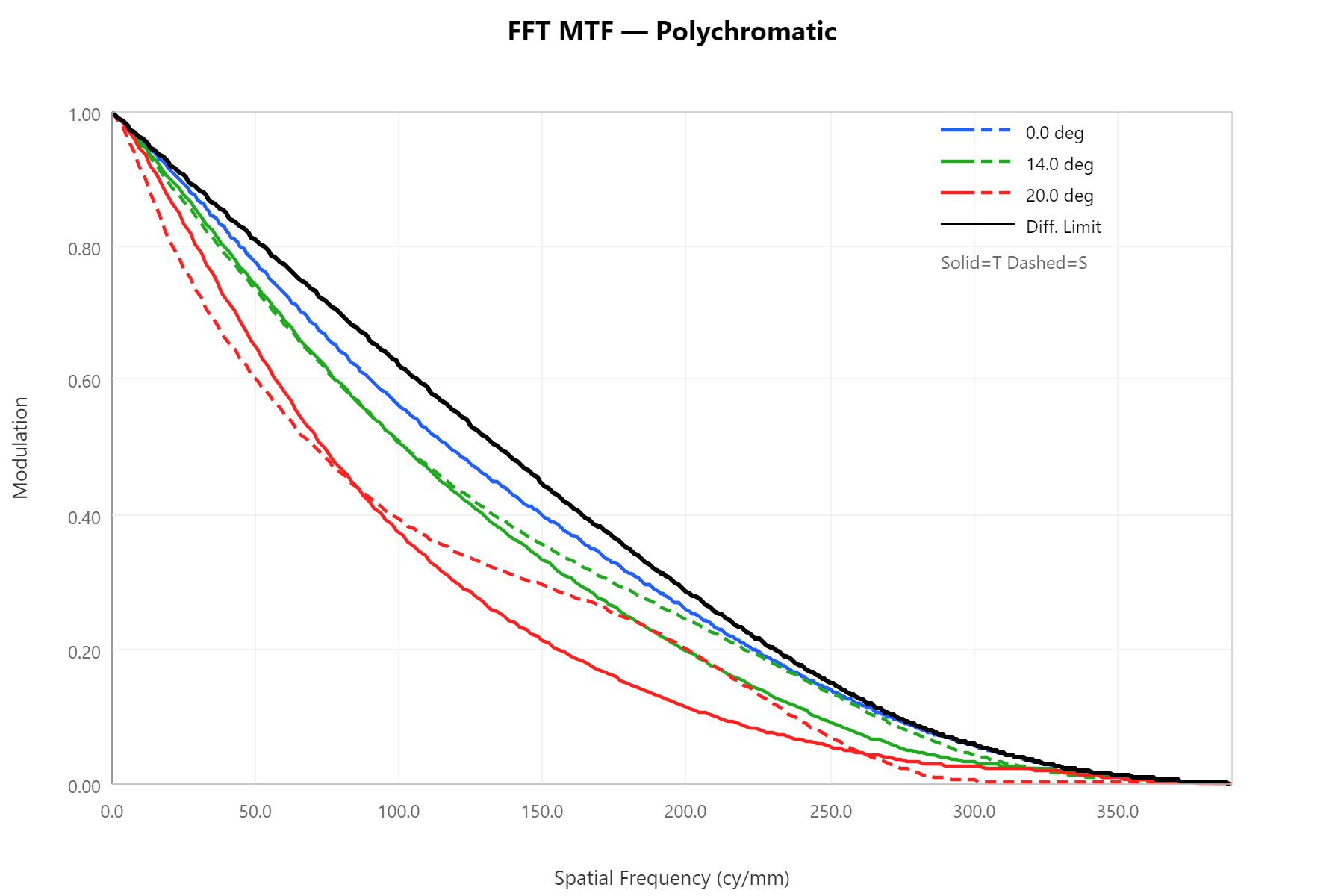 |
When to reach for Split Element:
- After Multistart / Basin Hopping have plateaued and Local LM finds no further improvement on the current topology.
- When the merit shows a clear residual aberration concentrated
on one element. The aberration scorer ranks all elements by
their summed
|S1|+|S2|+|S3|and picks the top one; you can see its choice in the log on every run. - When the design budget tolerates one more lens element — Split Element strictly adds a surface, never collapses one back.
What it isn't:
- A topology search. Split Element only refines around an existing topology by adding one surface at a time. To go from a doublet to a triplet, you'd run Split twice on different surfaces; to go from parallel plates to a Cooke triplet, run Multistart or Basin Hopping with glass substitution first.
Search Best Asphere Surface
Optimization → Search Best Asphere Surface…
Different way to add a degree of freedom: instead of inserting a new surface (Split Element), pick existing surfaces and turn them into even-aspheres. The dialog enumerates every glass surface, runs a short LM trial with that surface aspherized, ranks the surfaces by post-trial merit, applies the top-N changes permanently, and finishes with one final LM polish.
A run does four things in order:
- Enumerate candidate surfaces. Every glass surface is a
candidate (the log line
Candidate surfaces: 4 (1, 3, 5, 7)reports them). - Per-surface trial. For each candidate, the surface is
converted to Even Asphere with the selected coefficients (A4,
A6, A8) marked variable, then
LM/TrialLM iterations run. The post-trial merit and Δ % vs the starting merit are recorded; after each trial the surface is reverted. - Apply top N. Trials are ranked by post-trial merit and
the top
Top Nare applied permanently — those surfaces stay as Even Asphere with the LM-optimized coefficients. - Final LM polish (
Final LMiterations) runs on the composite design (now with N aspheric surfaces simultaneously variable) to pick up the cross-coupling gain.
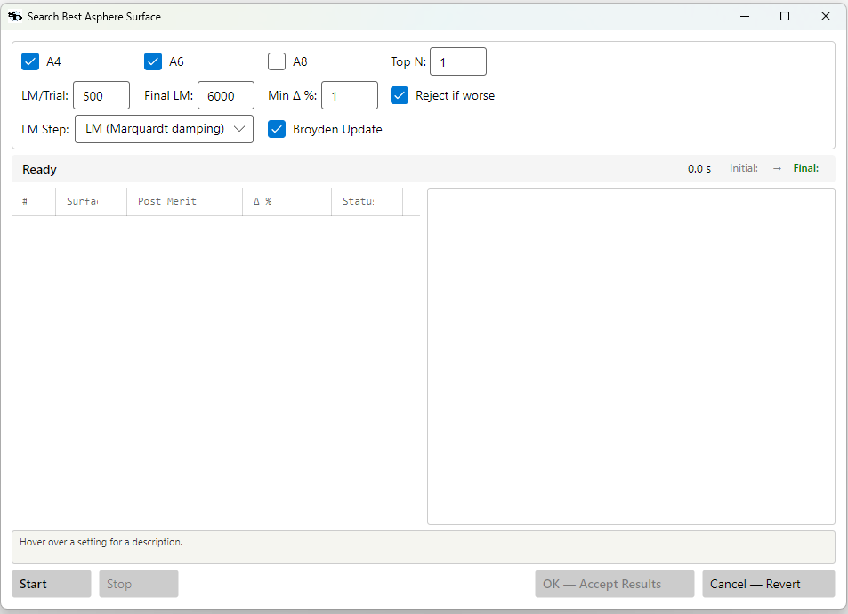
| Setting | Default | Meaning |
|---|---|---|
| A4 / A6 / A8 | A4, A6 on; A8 off | Which even-asphere coefficients to mark variable on each trial. A4 and A6 are on by default; enable A8 when a surface is working hard. Higher orders give finer correction but slower convergence and tighter manufacturability requirements. |
| Top N | 1 | How many of the ranked candidate surfaces to apply after the trial sweep. Default 1 = the single best surface; a larger N applies several for a composite improvement at the cost of more aspheric surfaces in the final design. |
| LM/Trial | 500 | LM iterations per per-surface trial. A short trial is enough to rank the candidates; the real polish happens in the Final LM step, so this stays small to keep the candidate × trial sweep fast. |
| Final LM | 6000 | LM iterations for the post-application polish across all newly aspheric surfaces. |
| Min Δ % | 1 | Minimum trial improvement (over the starting merit) required to consider a candidate surface. Trials below this are still listed in the table but the picker skips them when applying. |
| Reject if worse | on | If the post-final-LM merit is worse than the pre-search merit, the original geometry is restored. |
Why A4/A6/A8 and not the conic constant. The search fits the even-aspheric polynomial coefficients and deliberately holds the conic constant
kat 0. To lowest order the conic is degenerate with A4: the base conic's departure from a sphere is((1+k)/8)·c³·r⁴ + …— a term in r⁴, exactly what A4 controls. Free bothkand A4 and they push on the same handle, giving a rank-deficient, ill-conditioned fit. The conic's higher-order effect (r⁶, r⁸…) is itself a constrained subset of what A6/A8 already span, so once the polynomial is free the conic adds little but conditioning trouble. The polynomial is the more general parameterization, so it's the one the search uses — if a surface "wants" a strong conic, you'll see it show up as a large A4.
Case study: aspherizing a well-corrected Cooke triplet
Sample files (samples/UserGuide/LensFilesForManual/):
CookeTriplet_UC_GS_Best_BeforeAspherization.lhlt (start),
CookeTriplet_UC_GS_Best_AfterAspherization.lhlt, and
CookeTriplet_UC_GS_Best_AfterAspherization_AfterBasinHoppimg.lhlt.
The starting design is an already well-corrected Cooke triplet —
the best result of an earlier Basin-Hopping run — with a merit of
0.02627. The goal is to squeeze it further by aspherizing two
surfaces, then let Basin Hopping re-explore the glasses on the
aspheric design.
First: add intermediate fields
Before adding aspheres, widen the field sampling. This design was corrected on the usual three fields (0°, 14°, 20°), which is fine for all-spherical surfaces. But an even asphere adds several new degrees of freedom per surface, and the optimizer will happily spend them driving the merit down at the sampled fields — which can leave large gaps in between. The symptom is an MTF-vs-field curve that is excellent at 0 / 14 / 20° but sags badly at the un-sampled fields between them.
The remedy is to sample the field more densely before optimizing. Here the field set was expanded to seven points — 0, 5, 8, 11, 14, 17, 20° — so the optimizer has to keep every field honest:
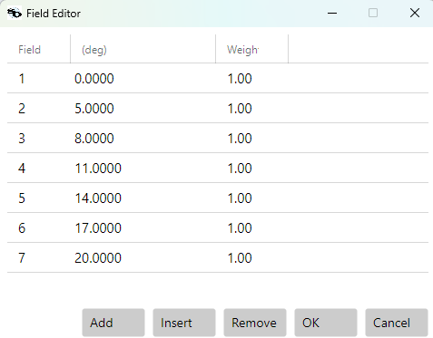
On this denser field set the starting design's merit is 0.02627.
The asphere search
Settings — A4 / A6 / A8 all on (A8 enabled manually), Top N = 2, LM/Trial = 500, Final LM = 6000, Min Δ % = 1, Reject if worse on:
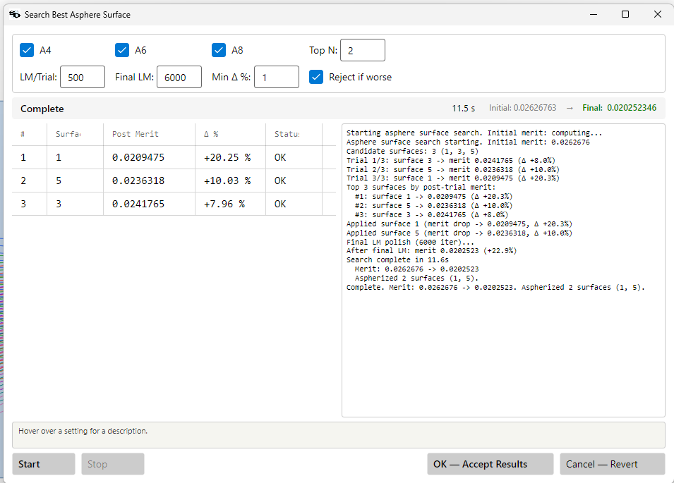
The candidate surfaces are the three glass front surfaces (1, 3, 5). The per-surface trial sweep (11.6 s) ranks them:
| # | Surface | Post-trial merit | Δ % |
|---|---|---|---|
| 1 | 1 | 0.020947 | +20.3 % |
| 2 | 5 | 0.023632 | +10.0 % |
| 3 | 3 | 0.024176 | +8.0 % |
With Top N = 2, surfaces 1 and 5 are aspherized; surface 3 is
left spherical. The final LM polish across the two new aspheric
surfaces takes the merit to 0.020252 — a +22.9 % reduction
from the 0.026268 start.
Follow-on: Basin Hopping on the aspheric design
This is exactly the workflow that used to abort before 1.0.137 — a global search on a design that already carries aspheric surfaces. It now runs to completion (see the release note for 1.0.137).
The aspherized design still uses the exotic glasses inherited from
the earlier optimization (S1 N-SF57, S3 LASF35, S5 N-PSK53A).
Running Basin Hopping with Glass substitution on and Glass
Source = CoreSet28 (a curated 28-glass, readily-manufacturable
set) lets it trade those for catalog glasses while re-tuning the
aspheric coefficients:
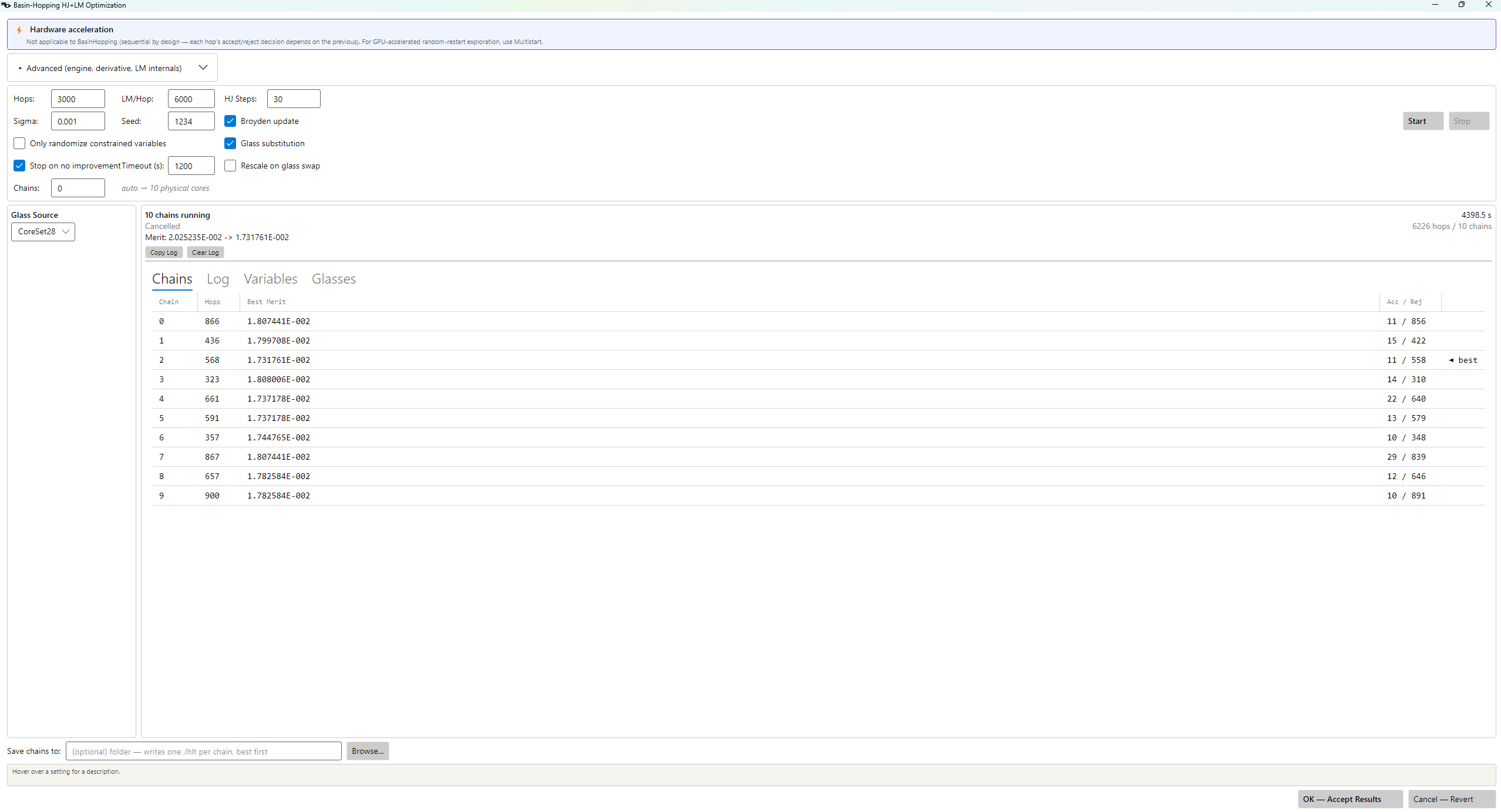
Settings — Hops 3000, LM/Hop 6000, HJ Steps 30, Sigma 0.001,
Broyden update on, 10 chains (auto), stop-on-no-improvement after
1200 s. The run stopped on the no-improvement timeout after 6226
hops across 10 chains (~73 min); the best chain (chain 2) reached
merit 0.017318 in 568 hops.
Result: merit 0.020252 → 0.017318 (a further −14.5 %). All three
glasses were swapped onto the CoreSet28 catalog —
N-SF57 → F2, LASF35 → SF2, N-PSK53A → N-PK51 — and both
aspheric surfaces (1, 5) were kept, with re-optimized coefficients.
Progression across the three stages
MTF vs field — the payoff from the denser field sampling: the response stays uniform across the whole field instead of sagging between the corrected points.
| Before | After asphere | After asphere + Basin Hopping |
|---|---|---|
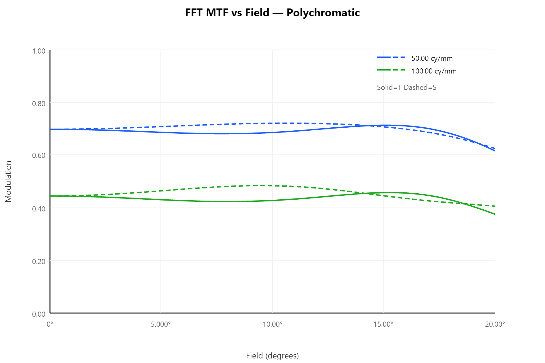 |
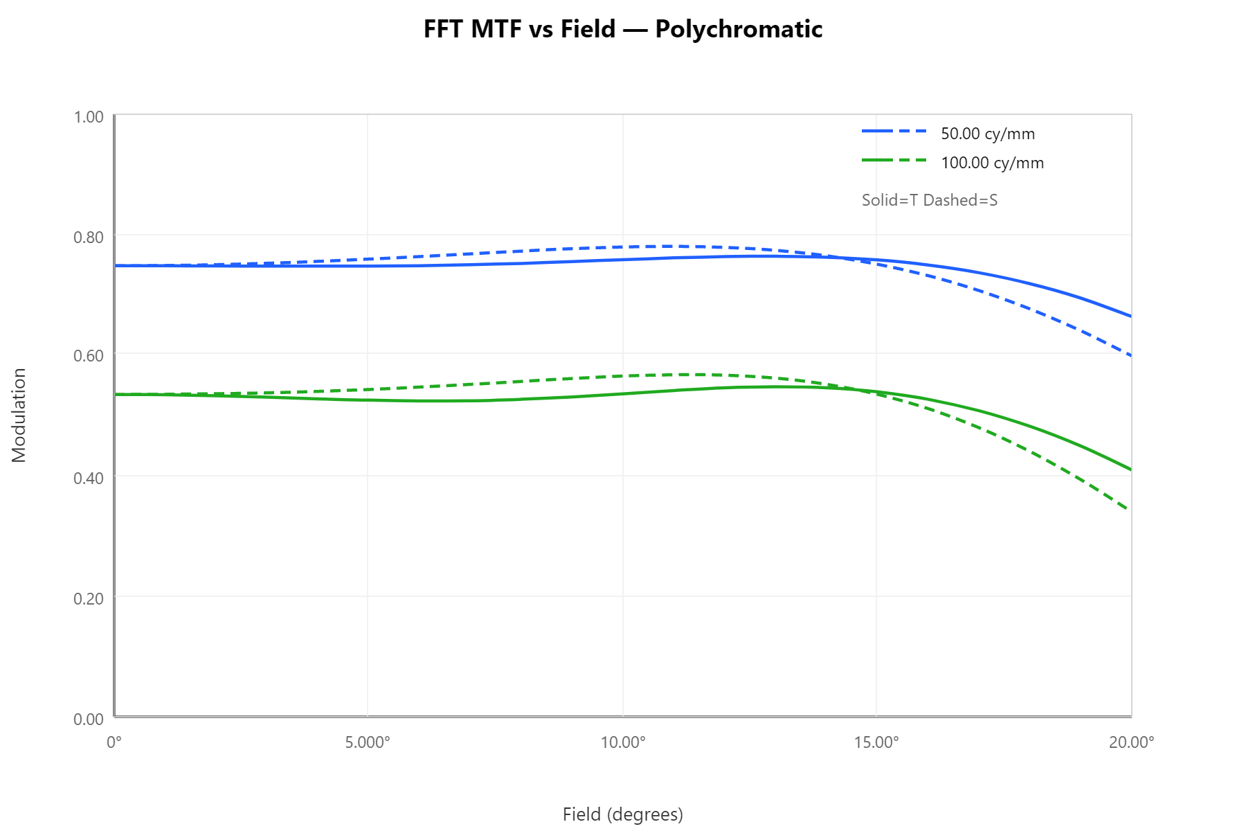 |
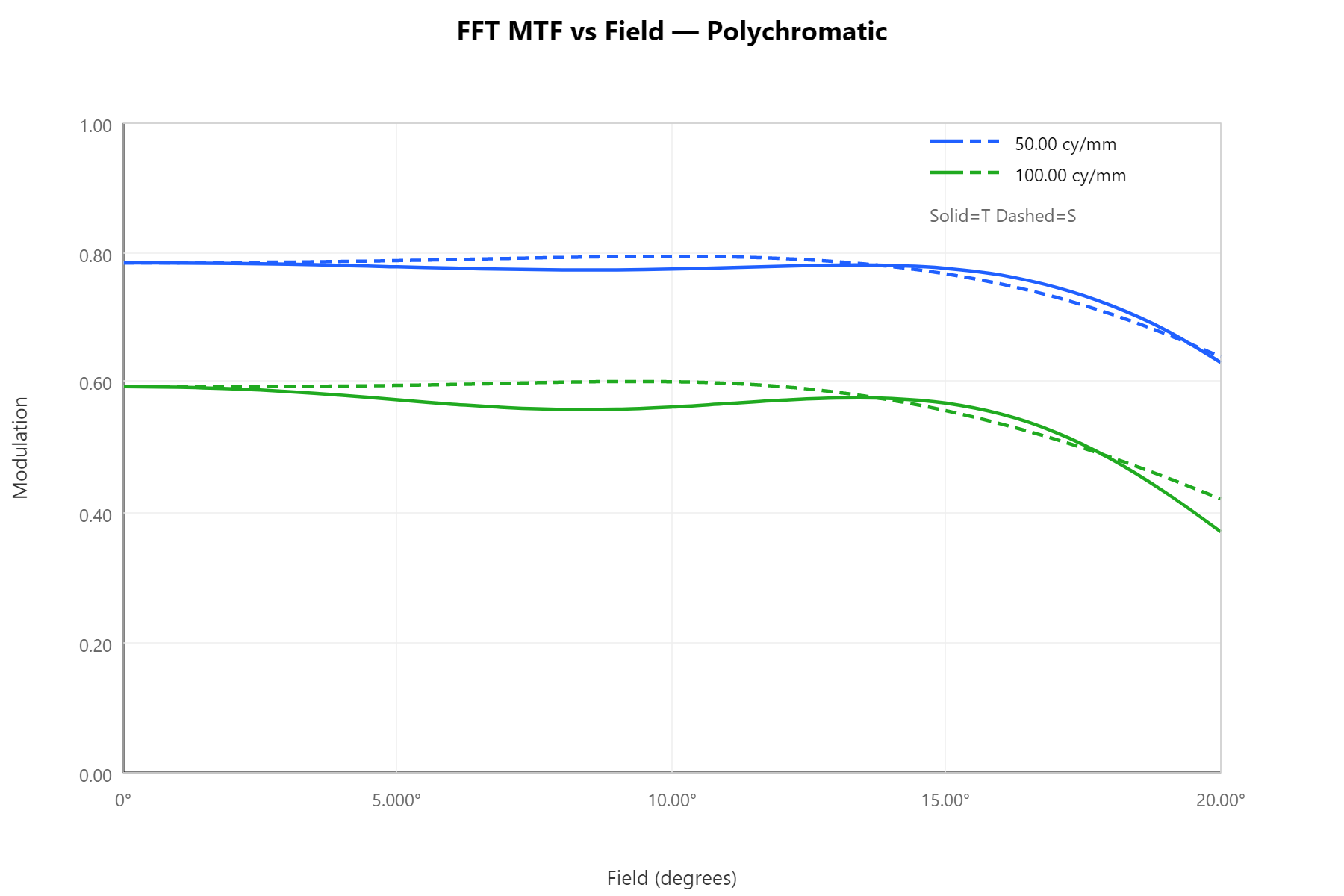 |
FFT MTF
| Before | After asphere | After asphere + Basin Hopping |
|---|---|---|
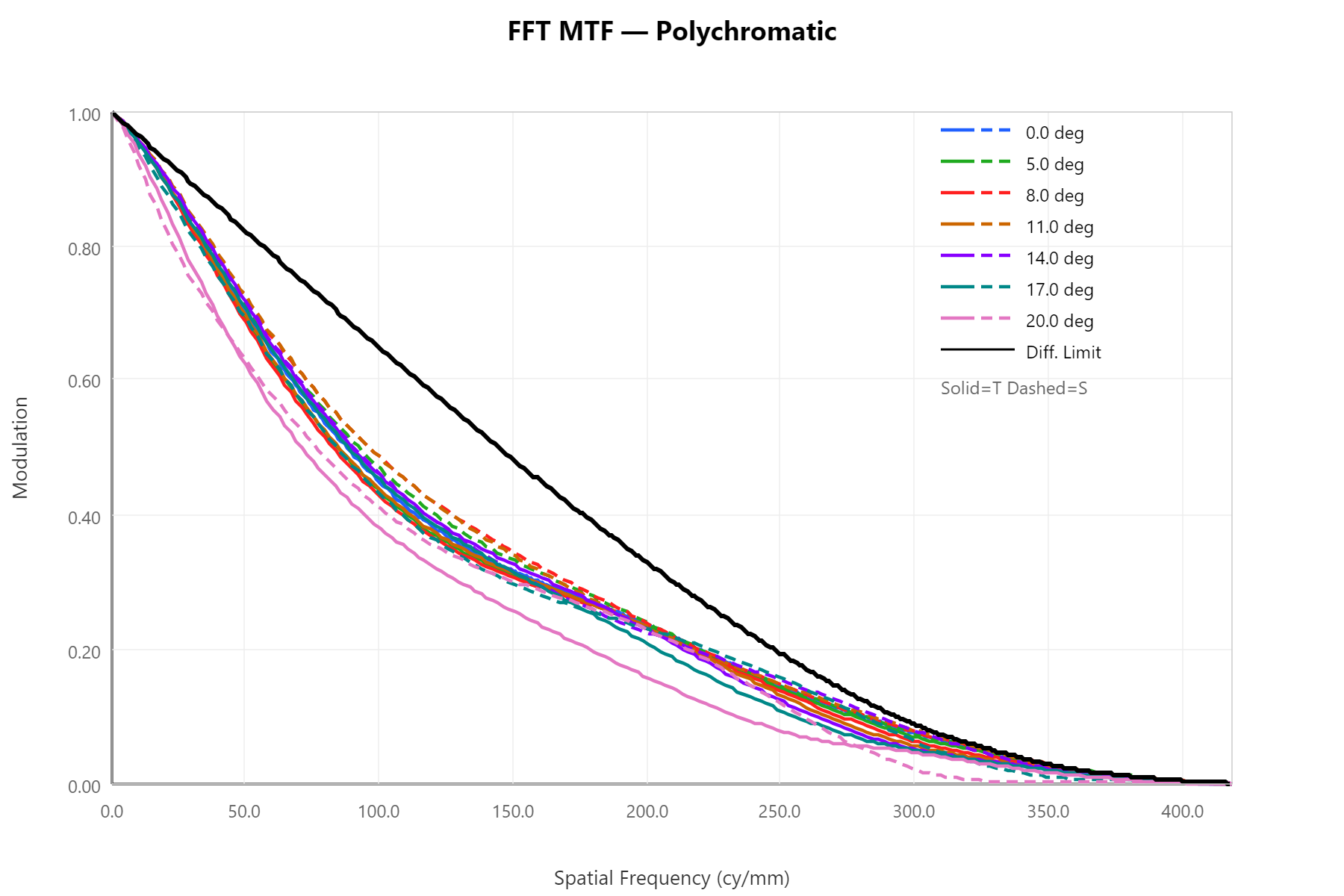 |
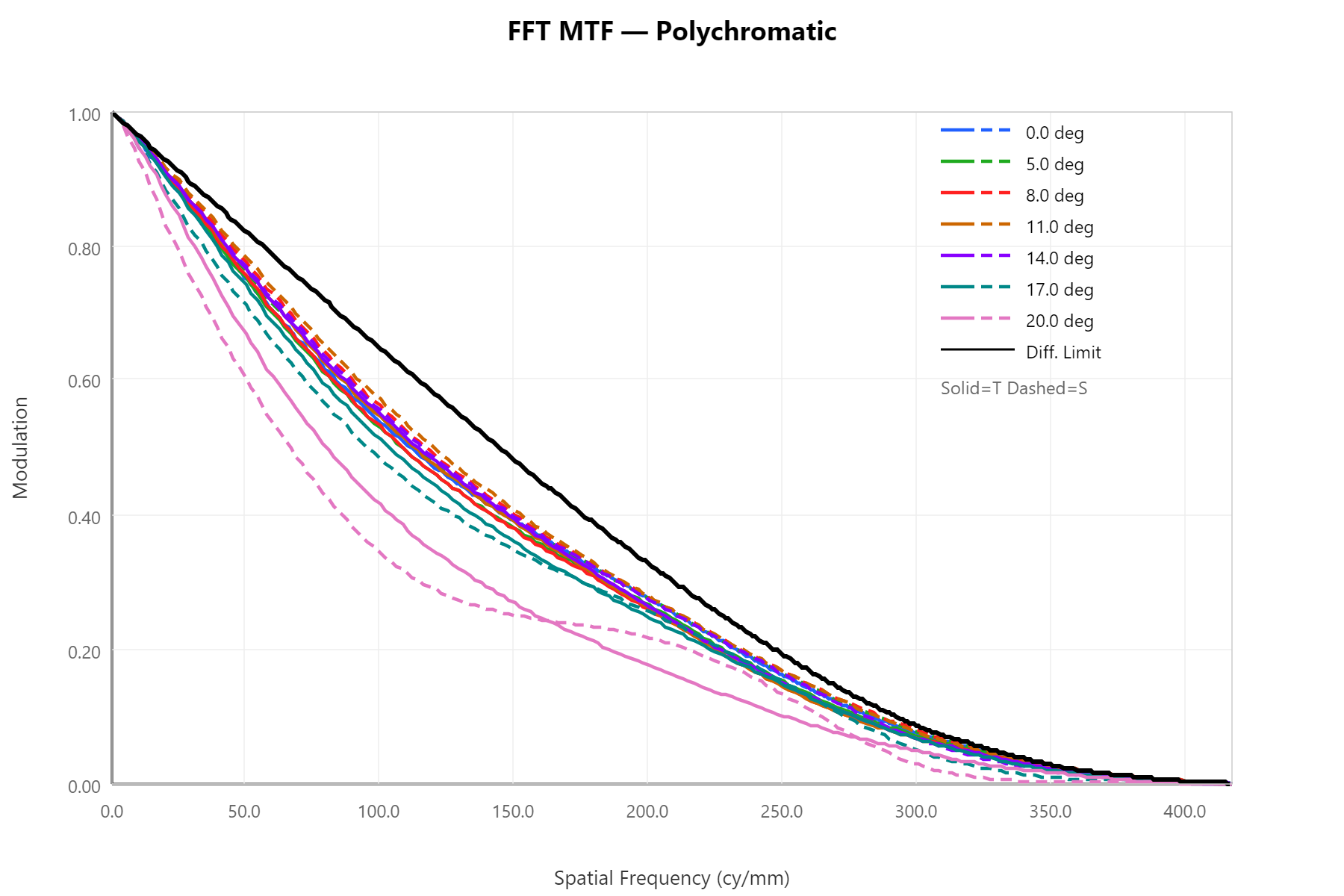 |
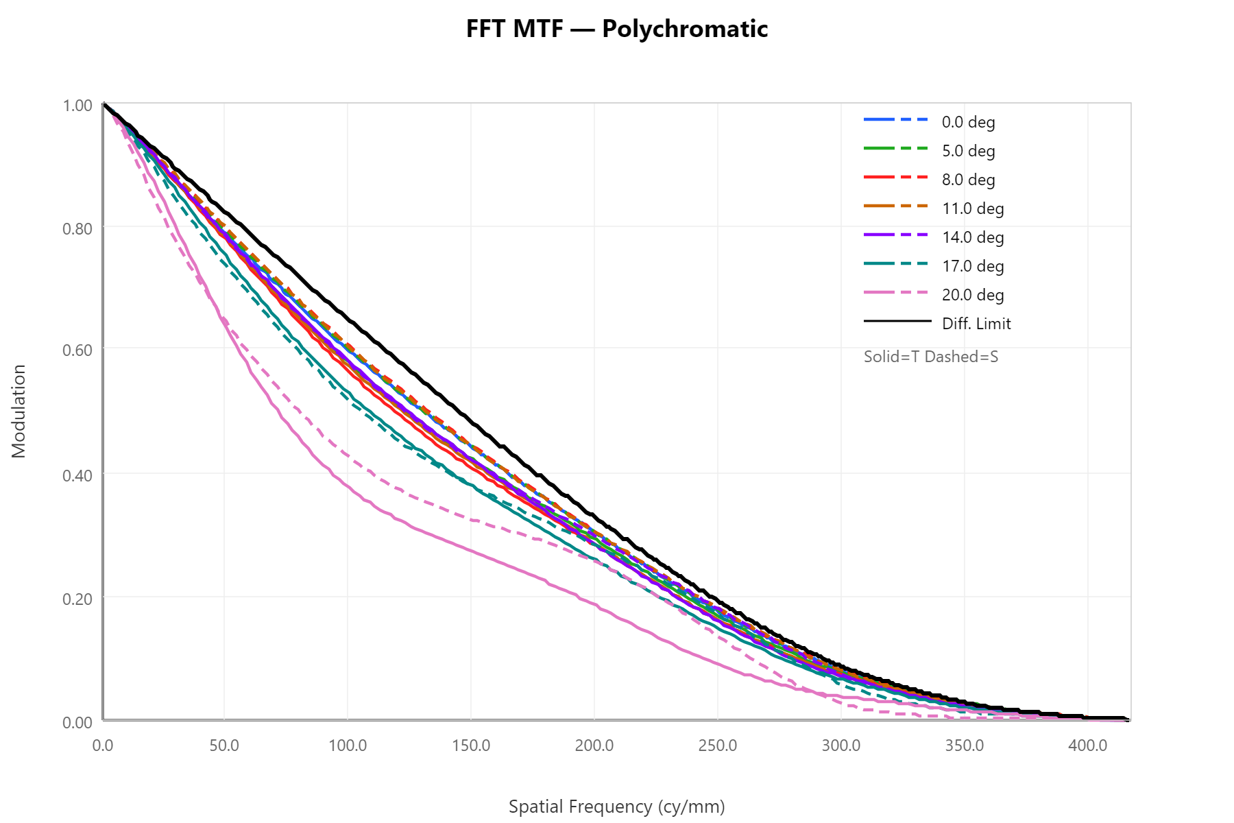 |
Spot size — RMS radius (µm), polychromatic
The spot radii are tabulated rather than shown as diagrams (the per-field spot images are hard to read at print size). Every field improves, and the two stages contribute in different places: the asphere does most of the work from the axis out to mid-field (8°: 2.97 → 2.17 µm), while Basin Hopping spends its remaining freedom on the outer field, where the asphere alone left the most on the table (17°: 4.02 → 3.09 µm; 20°: 6.17 → 5.30 µm). End to end the on-axis spot tightens from 3.15 to 2.73 µm and the 20° edge by ~30 %, from 7.62 to 5.30 µm — the outer field improving fastest is what keeps the MTF-vs-field curve flat.
| Field (°) | Before | After asphere | After asphere + BH |
|---|---|---|---|
| 0 | 3.15 | 2.83 | 2.73 |
| 5 | 3.09 | 2.54 | 2.55 |
| 8 | 2.97 | 2.17 | 2.28 |
| 11 | 2.86 | 1.99 | 1.94 |
| 14 | 3.20 | 2.55 | 1.94 |
| 17 | 4.72 | 4.02 | 3.09 |
| 20 | 7.62 | 6.17 | 5.30 |
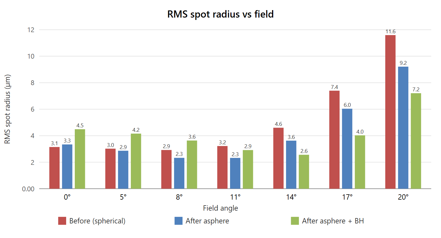
Wavefront map
| Before | After asphere | After asphere + Basin Hopping |
|---|---|---|
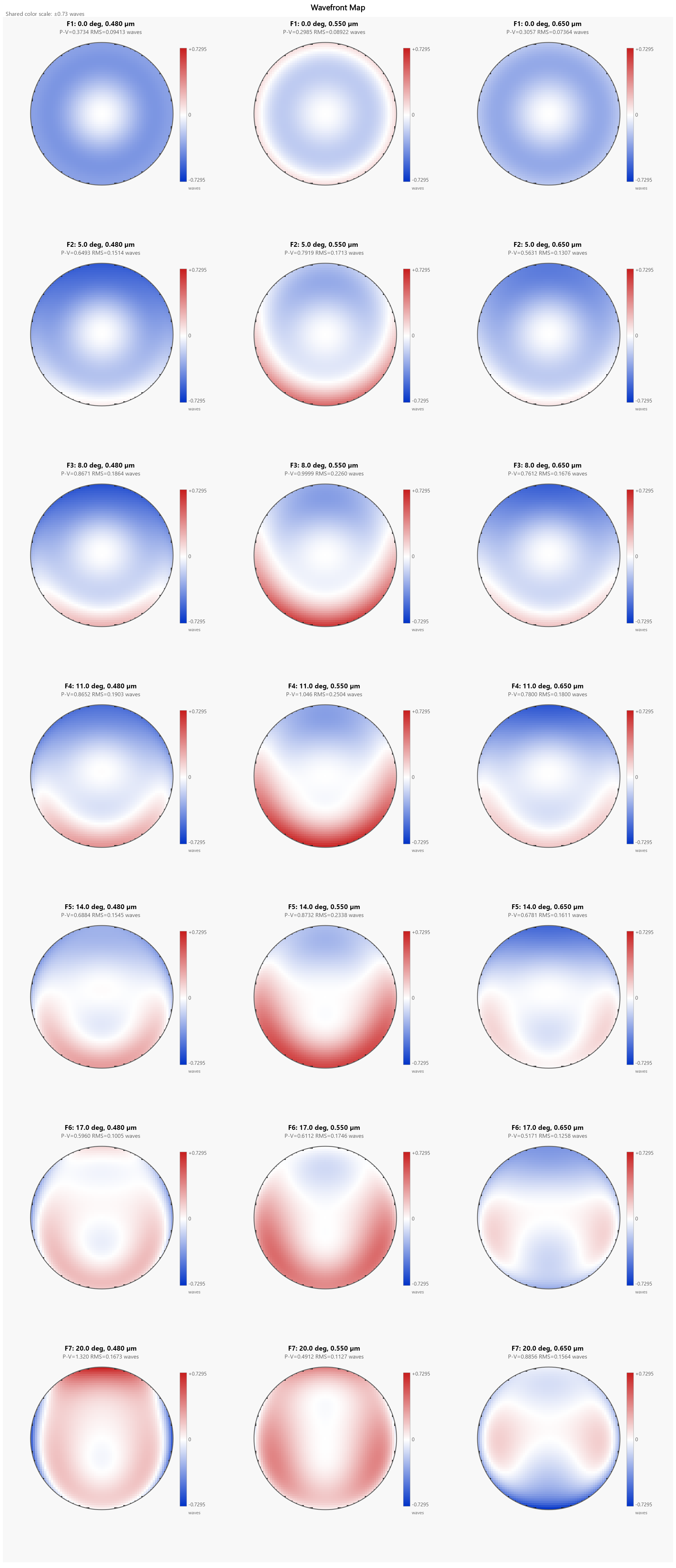 |
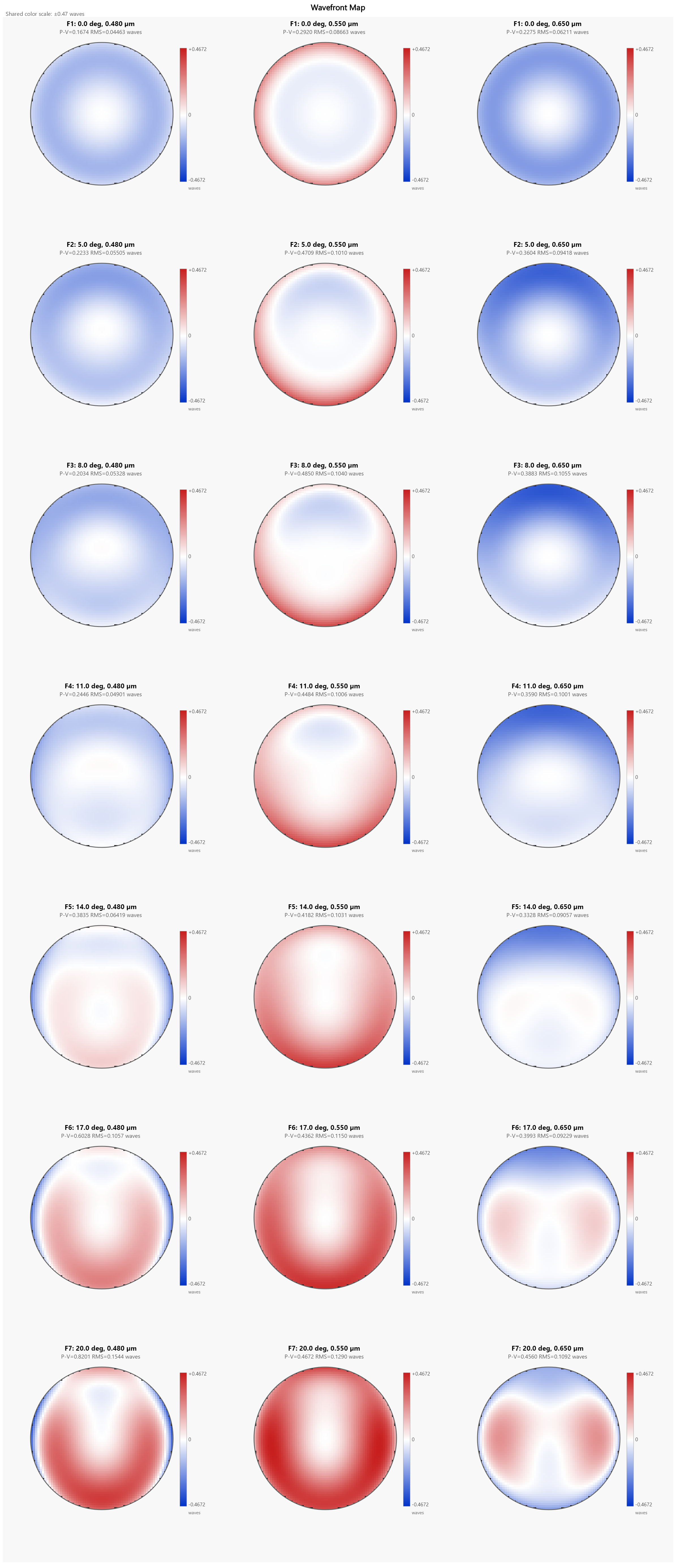 |
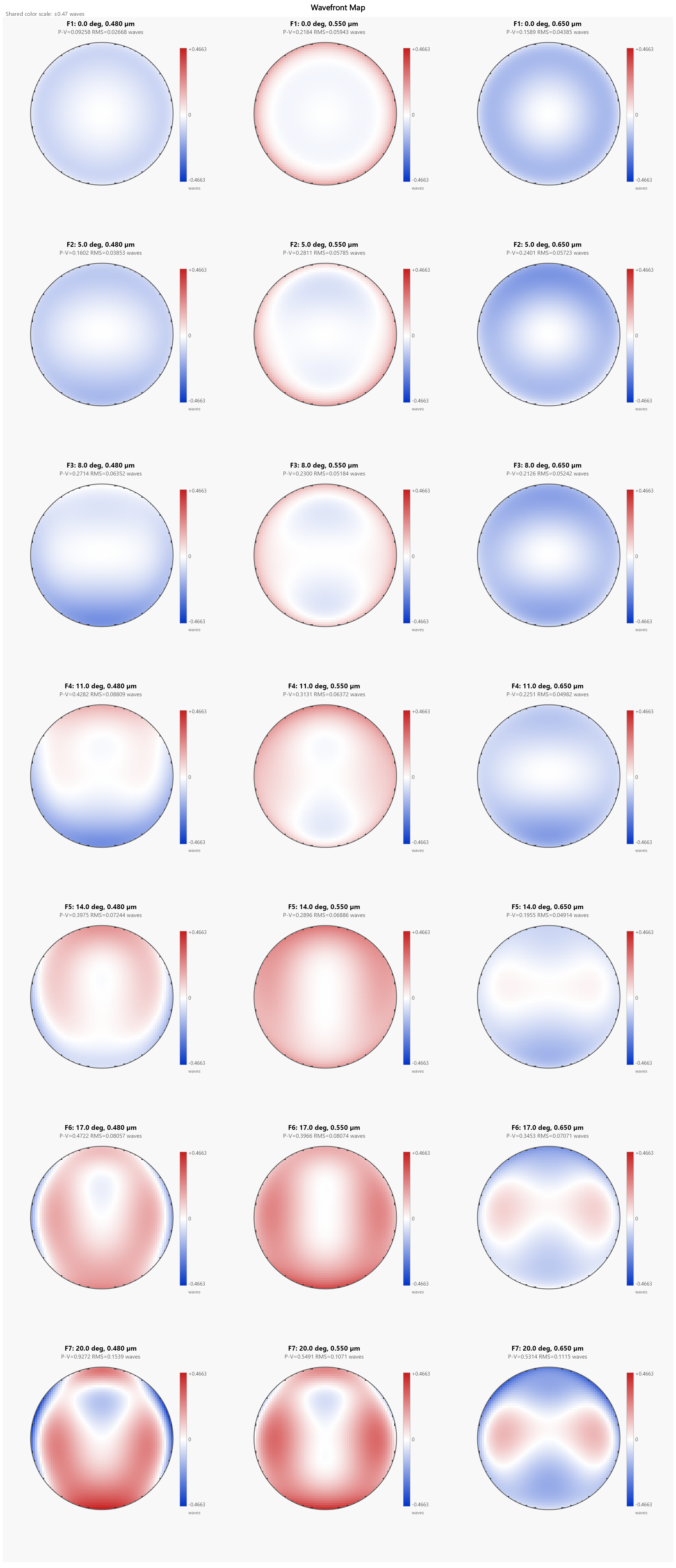 |
Wavefront error — RMS (waves), polychromatic
Weighted-RMS over the three lines (0.48 / 0.55 / 0.65 µm), the same convention as the merit function. The worst-field error falls from 0.209 to 0.126 waves and flattens across the field — the aspheres correct the mid-field zones, and the Basin-Hopping glass swap takes the on-axis error down to λ/22.
| Field (°) | Before | After asphere | After asphere + BH |
|---|---|---|---|
| 0 | 0.086 | 0.067 | 0.045 |
| 5 | 0.152 | 0.086 | 0.052 |
| 8 | 0.195 | 0.091 | 0.056 |
| 11 | 0.209 | 0.087 | 0.069 |
| 14 | 0.187 | 0.087 | 0.064 |
| 17 | 0.137 | 0.105 | 0.077 |
| 20 | 0.147 | 0.132 | 0.126 |
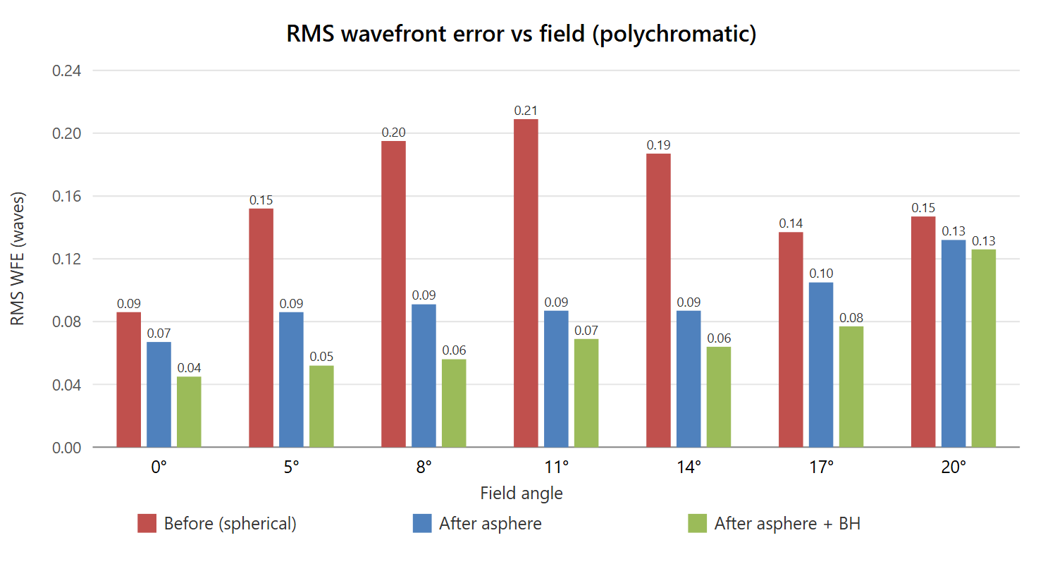
Layout
| Before | After asphere | After asphere + Basin Hopping |
|---|---|---|
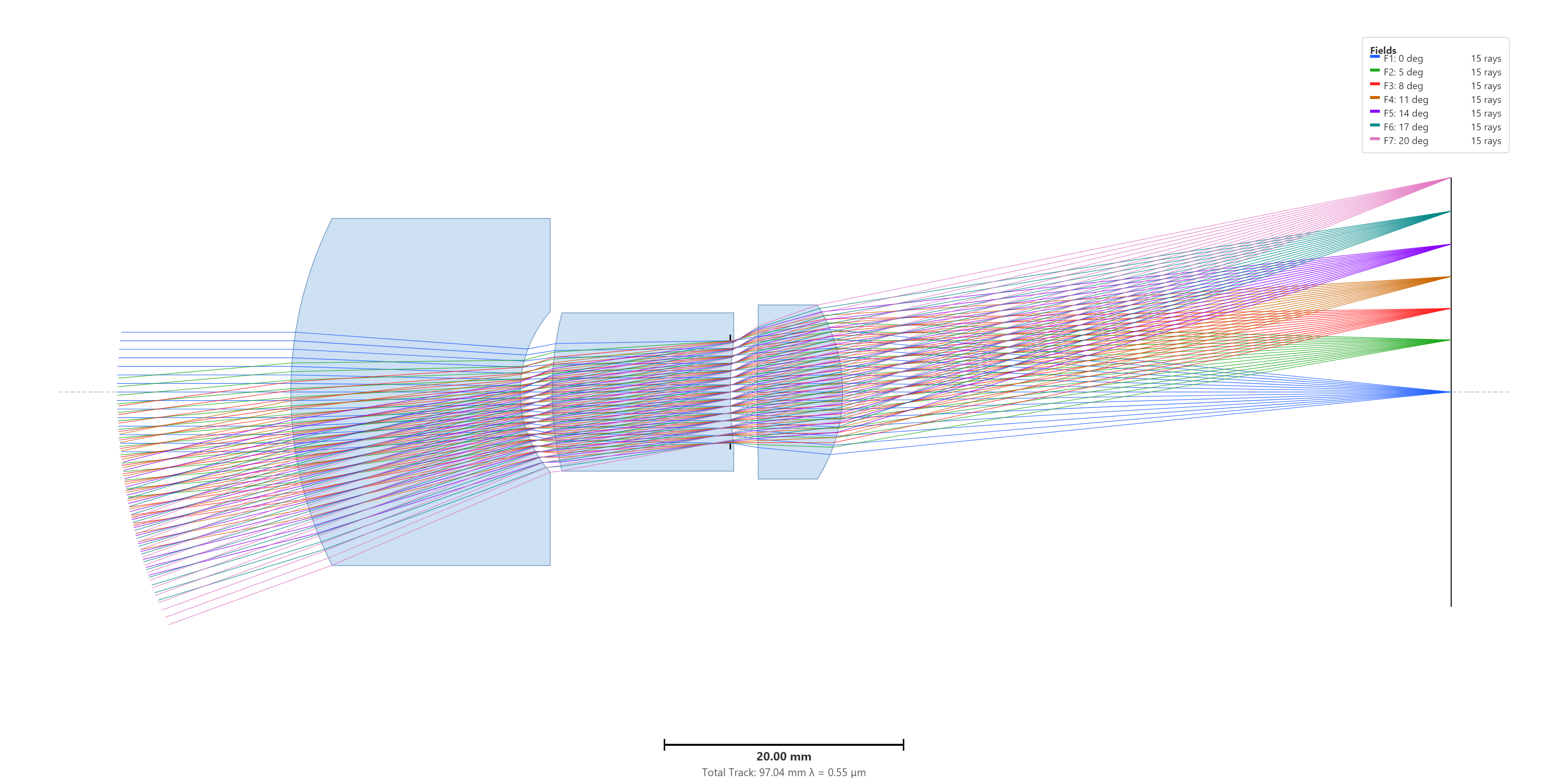 |
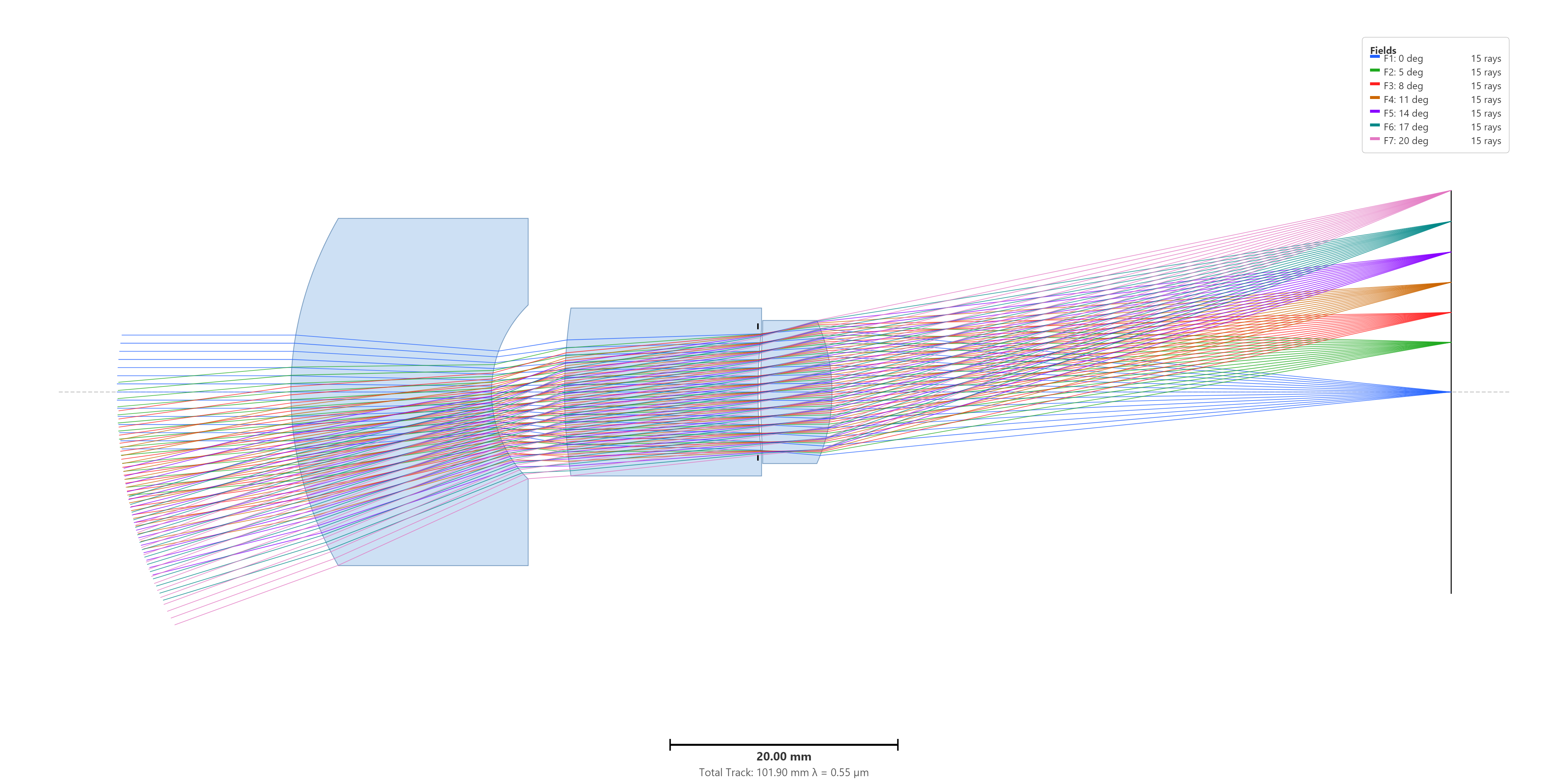 |
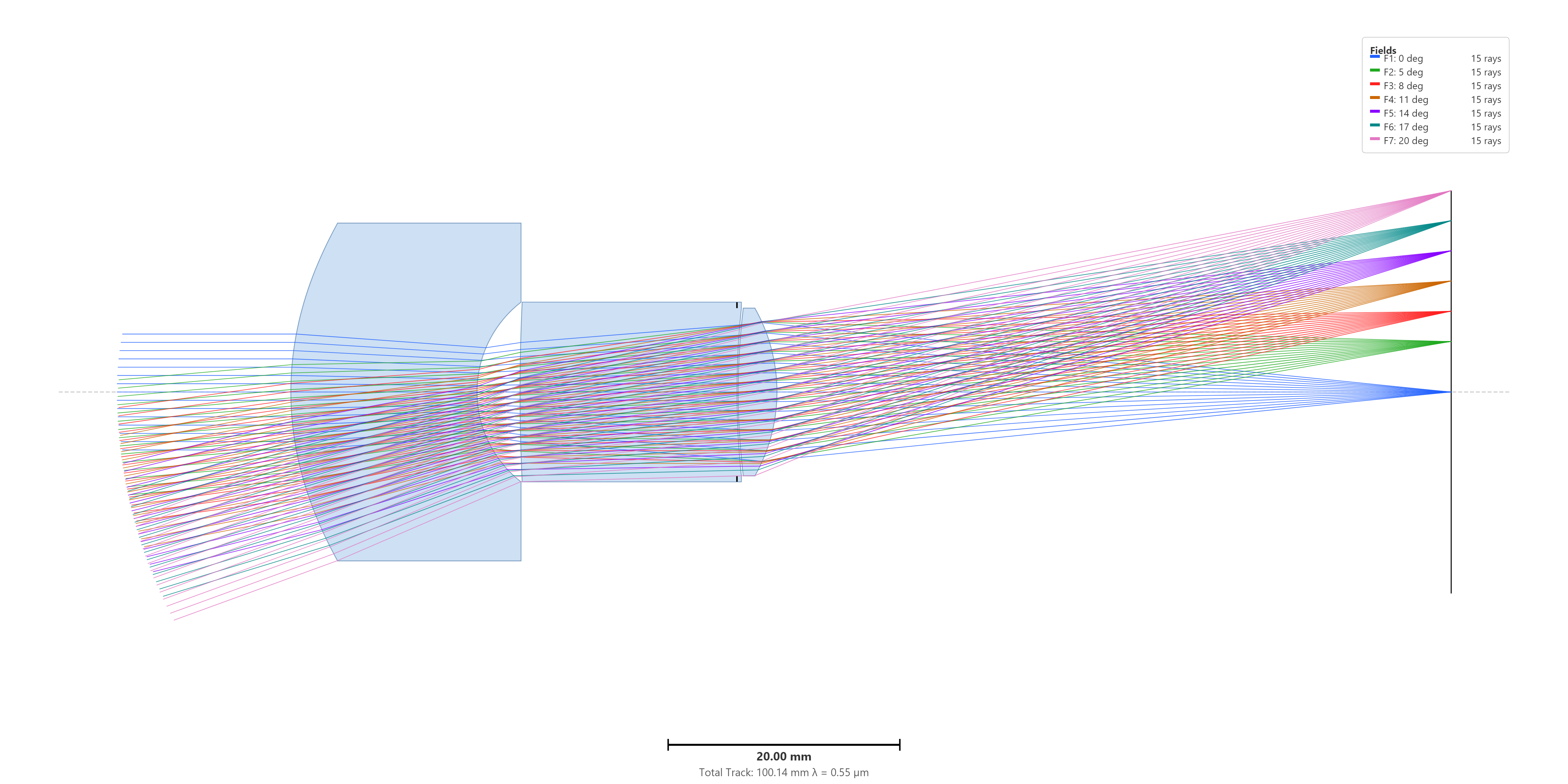 |
Net: the chain took the merit from 0.02627 (spherical) to
0.02025 (two aspheres) to 0.01732 (aspheres + a manufacturable
glass swap) — a 34 % reduction overall, and the final design
sits on catalog glasses. Two practical notes:
- Aspheric surfaces are not free to fabricate. Keep Top N as low as the design allows — here two surfaces bought the bulk of the gain, and surface 3 was left spherical on purpose.
- Add fields before you add degrees of freedom. The extra aspheric coefficients make it easy to over-fit the sampled fields; the denser 7-field set is what keeps the MTF-vs-field curve uniform through the whole image.
SPC (Synthesis by Saddle-Point Construction)
Optimization → Synthesis by SPC…
A topology generator. SPC grows a design one element at a time by finding saddle points in merit-vs-curvature space and branching off them — perturbing the saddle in either direction spawns two distinct local minima, and the better of each pair becomes the seed for the next round. Where Multistart and Basin Hopping shuffle parameters within an existing topology and Split Element grows a topology by one surface per call, SPC is the only tool in the box that can grow a design from a single lens to an arbitrary multi-element topology in one run.
The method follows Hou et al., Optics Express 24, 21 (2016).
A run does five things per level (one new element added per level):
- Pick insertion positions. Every air gap in every surviving parent design is a candidate. The Insert side dropdown can restrict to pre-stop only (objective-style) or post-stop only (eyepiece-style); default is both sides.
- Insert a near-zero null element. A glass element that is optically inert (front and rear curvatures equal, infinitesimal thickness) is dropped into the air gap. The merit jumps because the bootstrap penalty grows the null element to a real thickness.
- Scan curvature for saddles. The shared front+rear curvature
is swept across
[Scan c-min, Scan c-max]inStepssamples. Saddle points — where the merit's first derivative changes sign non-monotonically — become the branch seeds. - Perturb and optimize. Each saddle spawns two branches (
+εand−εperturbations of the curvature). A bootstrap LM grows the null element aboveMin Glass, then a full LM runs on each branch. After convergence, glass trials swap in random glasses (or glass pairs for cemented doublets) and re-optimize. - Prune to Top-N. All branches are ranked by final merit and
the best
Top Nsurvive to seed the next level.
Element topology
The Element dropdown picks what gets inserted at each saddle:
- Single — one glass element with two surfaces (the original Hou paper formulation). Cheapest per candidate.
- Cemented Doublet — three surfaces (front-glass A, cemented A-B interface, back-glass B). The saddle scan locks all three curvatures together so the seed remains a null element; glass trials enumerate (A,B) pairs and the post-saddle LM relaxes the doublet into an achromat. The crown glass comes from Null glass and the flint partner from Flint glass (defaults N-BK7 + SF5). Seeding both surfaces with the same glass collapses the doublet to a single thicker block during the scan, which is why a real flint partner is required from the start.
- Single + Cemented Doublet — runs both topologies at every position; the Top-N ranking picks the best across topologies. Roughly 2× the per-position compute cost. Modes that include doublets auto-drop Top N from 5 to 3 because doublet candidates are much more expensive to optimize.
Max Elements counts insertions, not lens elements — a doublet
counts as one insertion but two lenses. With Max Elements = 2 in
"Single + Cemented Doublet" mode the result can be 2 singlets,
2 doublets (4 lenses), or 1 of each (3 lenses), depending on which
the Top-N ranking picks at each level.
Selected settings
| Setting | Default | Meaning |
|---|---|---|
| Max Elements | 2 | Number of insertion levels. Each level adds one element (single = 1 lens, doublet = 2 lenses). |
| Top N | 5 (3 if doublets enabled) | Branches kept per level. Higher → broader search; lower → faster. |
| Threads | CPU cores | Outer-parallel branch evaluation. |
| Scan c-min / c-max | −0.1 / +0.1 | Curvature scan range applied to the inserted surface. Widen if the log reports saddles outside the range. |
| Steps | 100 | Samples between c-min and c-max. |
| Glass Trials | 50 | Random glasses (or pairs) tried per branch after the geometry converges. |
| LM/Trial | 4000 | Per-glass-trial LM iteration cap. |
| Min Glass / Max Glass | 1 / 25 mm | Centre-thickness bounds applied to inserted glass elements. |
| Min Air / Max Air | 0.1 / 50 mm | Air-gap bounds. |
| Min Edge | 1 mm | Edge-thickness floor enforced via EG/EA operands. |
| Post LM | 4000 | Final LM after the glass trials on each surviving branch. |
| Insert side | Both | Restrict insertions to pre-stop or post-stop air gaps. |
| Element | Single | Topology of each new insertion (see above). |
| Null glass / Flint glass | N-BK7 / SF5 | Crown / flint seed for the inserted element. The trial phase replaces these later. |
| Glass Source | first filtered catalog | Glass pool for the trial phase. |
Constraining proportions: the DTRG operand
SPC is unusually willing to make extreme element shapes — the
saddle scan happily lands on configurations with a wafer-thin
meniscus or a brick-thick block if those locally minimize the
image-quality residuals. The EG / EA operands keep edges
above a floor, but they don't prevent the centre from growing
absurd relative to the lens diameter.
The fix is the DTRG operand (Diameter-to-Thickness Ratio,
Glass-only) — see Merit Function § Boundary operands.
DTRG = 2·SD / |CT|; bounding it to roughly [2, 10] enforces
fabricable proportions: the centre thickness can be at most half
the diameter (no super-thick blocks) and at least one tenth of the
diameter (no wafer lenses). One row covering the inserted-element
range with weight 0.3 is enough — the case study below uses it.
Case study: BK7 singlet → 3-element design (singlet + doublet)
Sample folder: samples/UserGuide/SingletBK7SPC/. The
starting design is a single biconvex N-BK7 element (50 mm EFL,
F/4, 12.5 mm entrance pupil, fields 0/7/10°, three visible wavelengths).
Glass substitution is enabled on S1 against the S1_GLASS
filtered catalog. The merit function carries the full boundary
set — EG, EA, CTG, CTA plus an explicit BFL operand —
and a DTRG row with weight 0.3, bounds [2, 10], covering
the inserted-element span.
| Before — single biconvex BK7 | After — singlet + cemented doublet around the stop |
|---|---|
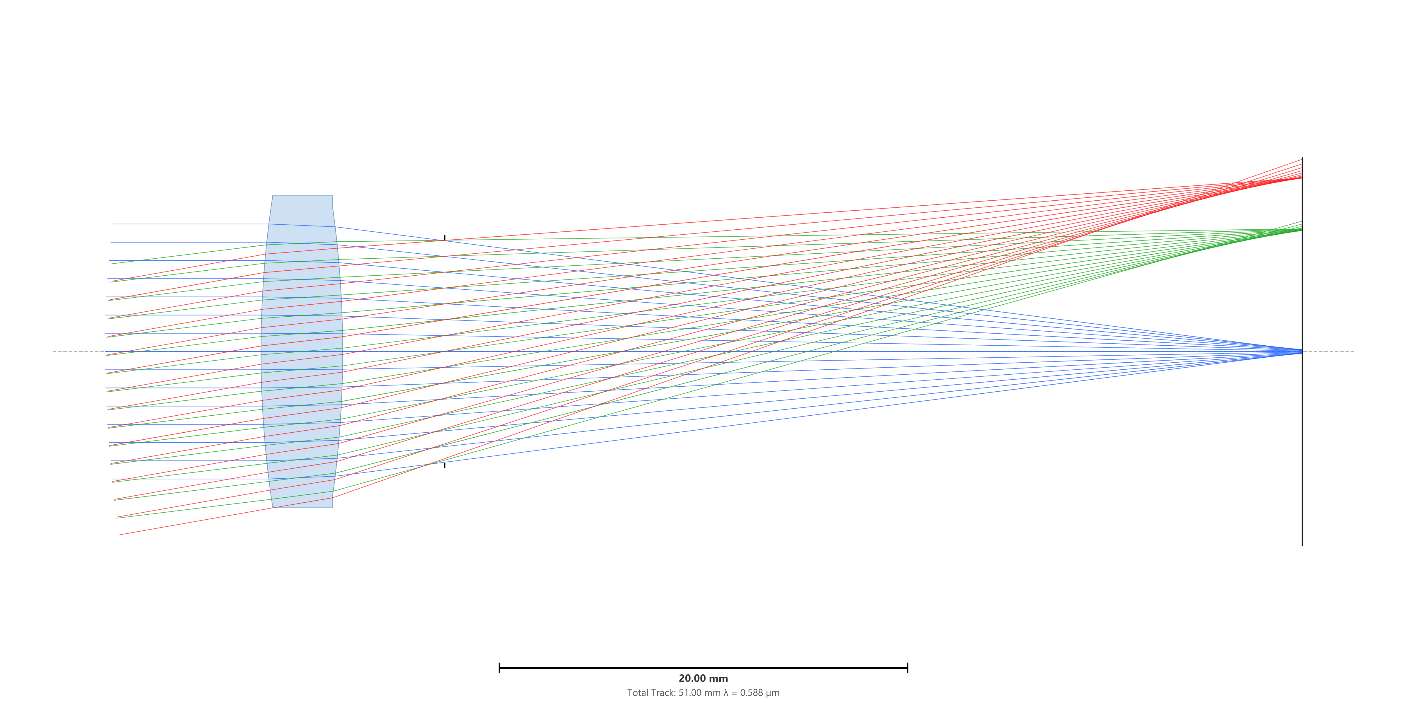 |
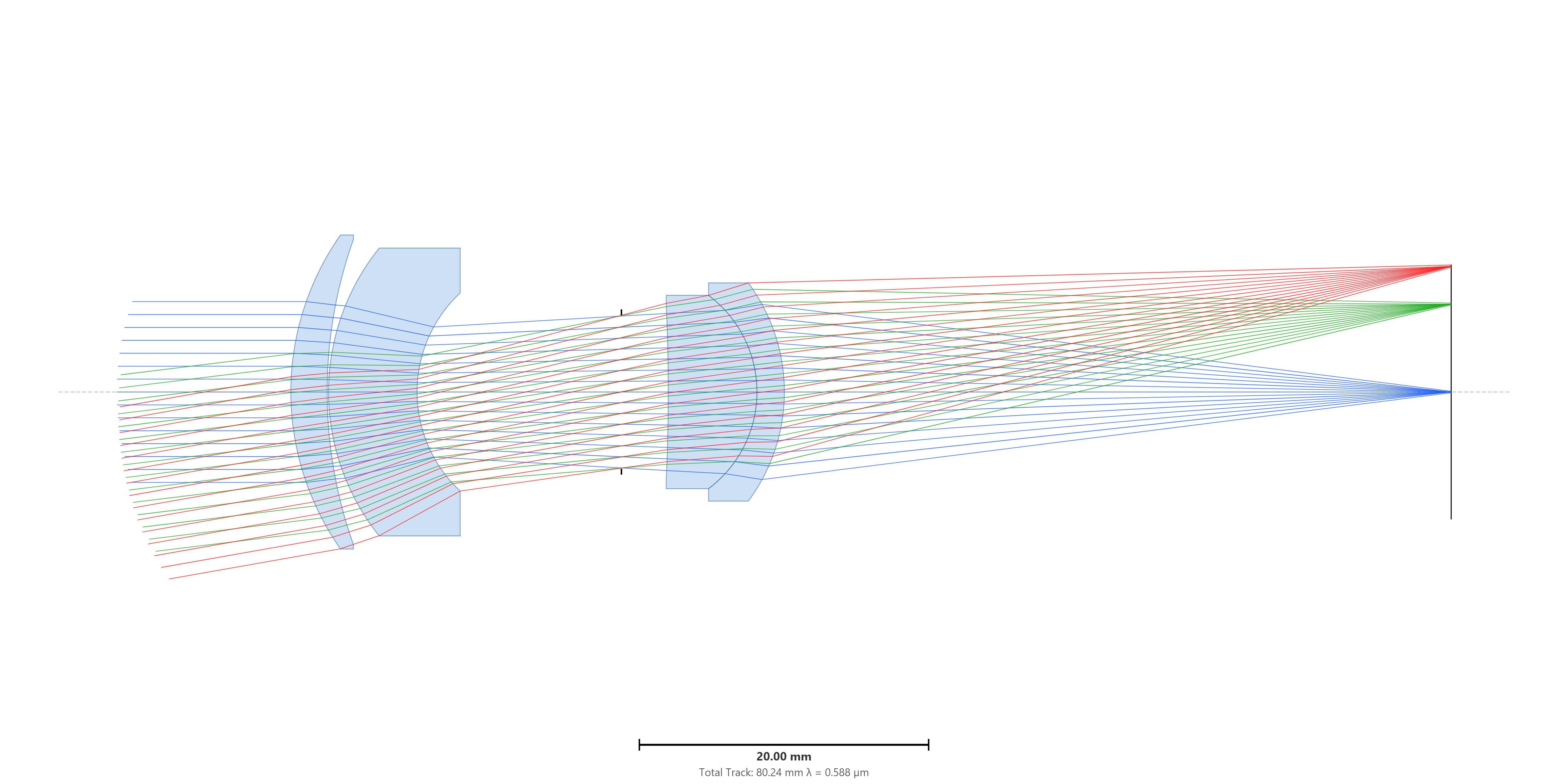 |
The starting merit function — note the DTRG row (#7, weight
0.3, bounds 2-10, span S1-S3) and the dedicated BFL CTA row
(#8, S3 only, min 40 mm). Boundary operands span the full
inserted range so SPC's geometry stays manufacturable as the
design grows:
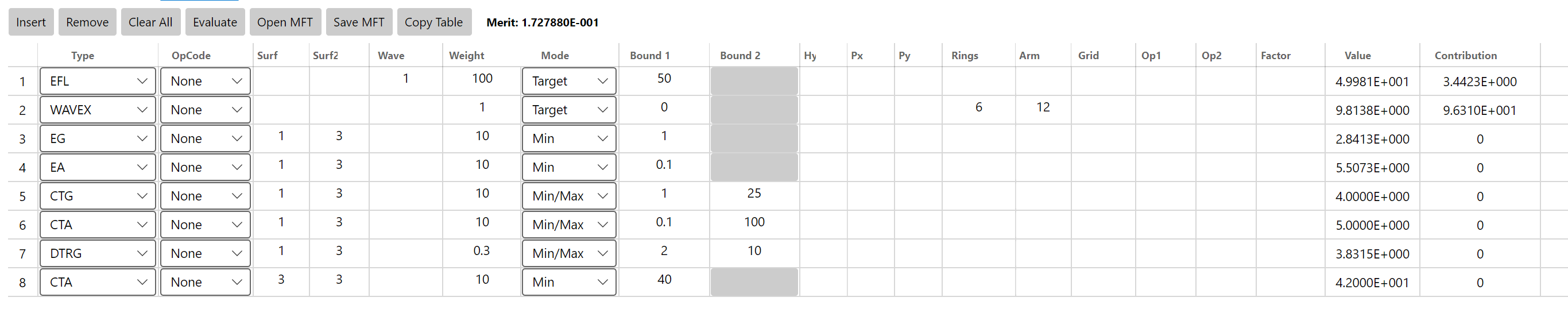
Settings used:
Max Elements = 2, Element = Single + Cemented Doublet,
Top N = 3 (auto-set when doublets are enabled), Glass Source = CoreSet28. The two non-default knobs that mattered: Scan
range widened to ±0.2 and Steps raised to 200 — the BK7 starting
design has surface curvatures around ±0.02 mm⁻¹, but the saddles
the SPC method needs to find sit out near ±0.1 (you can see this
in the L2 BEST line: c = 0.0671). Default ±0.1 would have
clipped half of them; doubling the range and the steps keeps the
sample density matched.
The Top-N ranking picked one single insertion at one level and one cemented doublet at the other — exactly the mix the "Both" topology mode is designed to surface.
The trajectory from the log:
| Phase | Best merit | Note |
|---|---|---|
| Start | 0.925 | Biconvex BK7, severe spherical + chromatic. |
| L1 BEST | 0.0192 | First insertion (a singlet on the pre-stop side). ~48× drop. |
| L2 BEST | 0.00622 | Second insertion (a cemented doublet on the post-stop side), best pair from glass trials. SPC output. |
| + Multistart pass | 0.00434 | Multistart with glass substitution on every glass surface; 23 / 648 trials accepted, merit 6.22 × 10⁻³ → 4.34 × 10⁻³ (~30 % further drop). Three of the four glass picks changed in the process — S1: N-BK7 → N-FK58, S3: LASF35 → SF4, S7: LAFN7 → N-BASF2 — so Multistart was both refining curvatures and finding a better glass combination than SPC's per-branch glass trials had landed on. |
Net: merit 0.925 → 4.34 × 10⁻³ — a ~210× reduction from a
single-element starting point in two SPC levels plus a Multistart
polish. Final topology: N-FK58 meniscus + SF4 element pre-stop,
then a N-BK7 + N-BASF2 cemented doublet post-stop.
| Spot after SPC | Spot after SPC + Multistart |
|---|---|
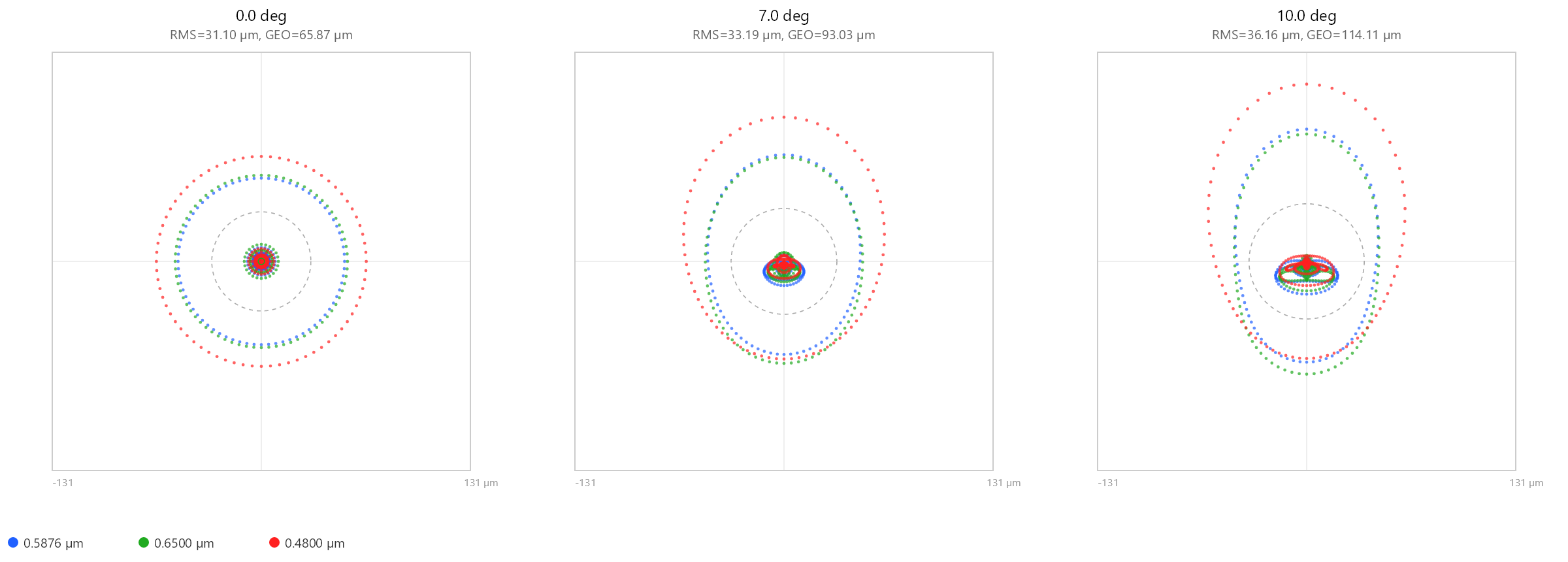 |
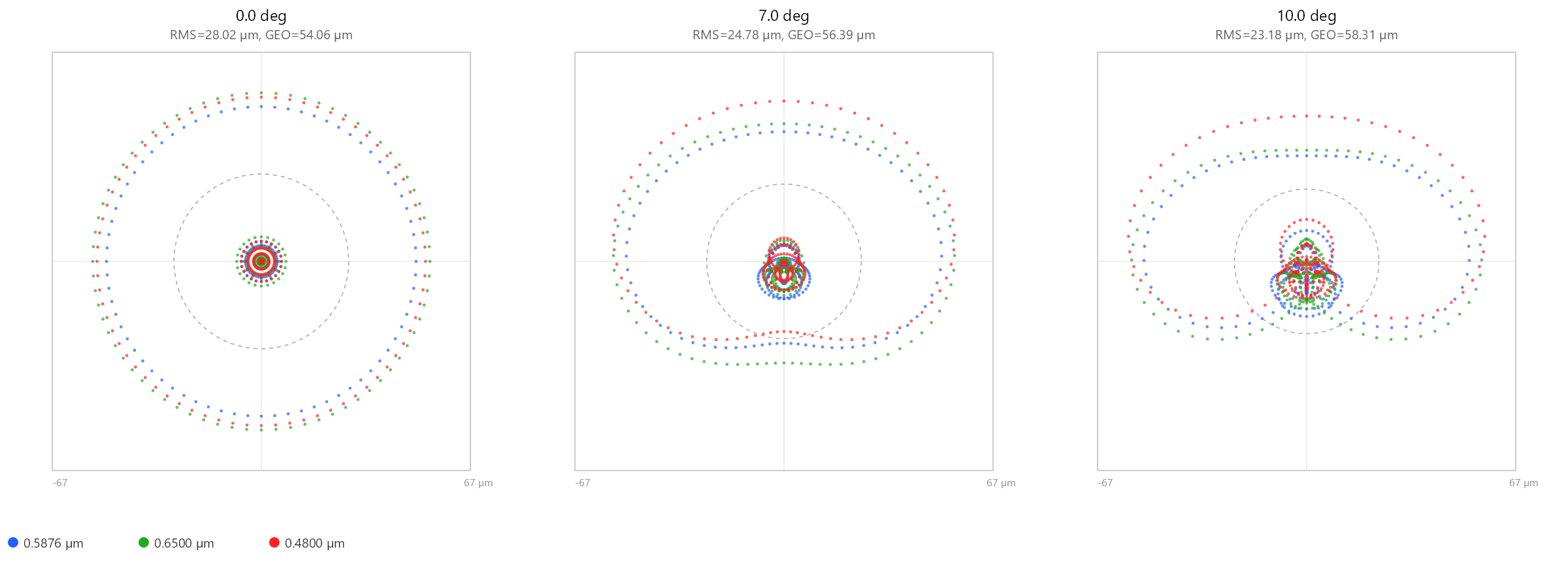 |
| FFT MTF after SPC | FFT MTF after SPC + Multistart |
|---|---|
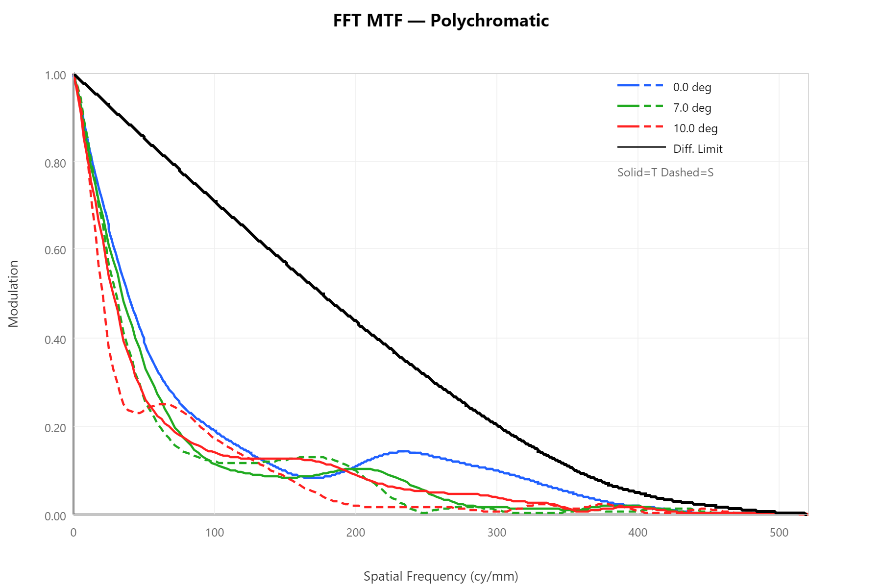 |
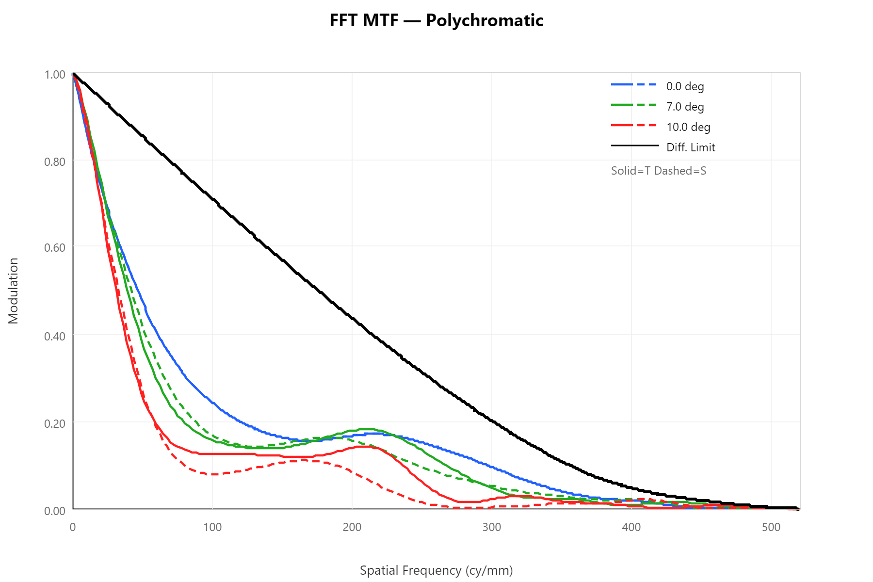 |
The follow-on Multistart dialog — initial merit 6.22 × 10⁻³
(SPC output) → best 4.34 × 10⁻³, 23 of 648 trials accepted:
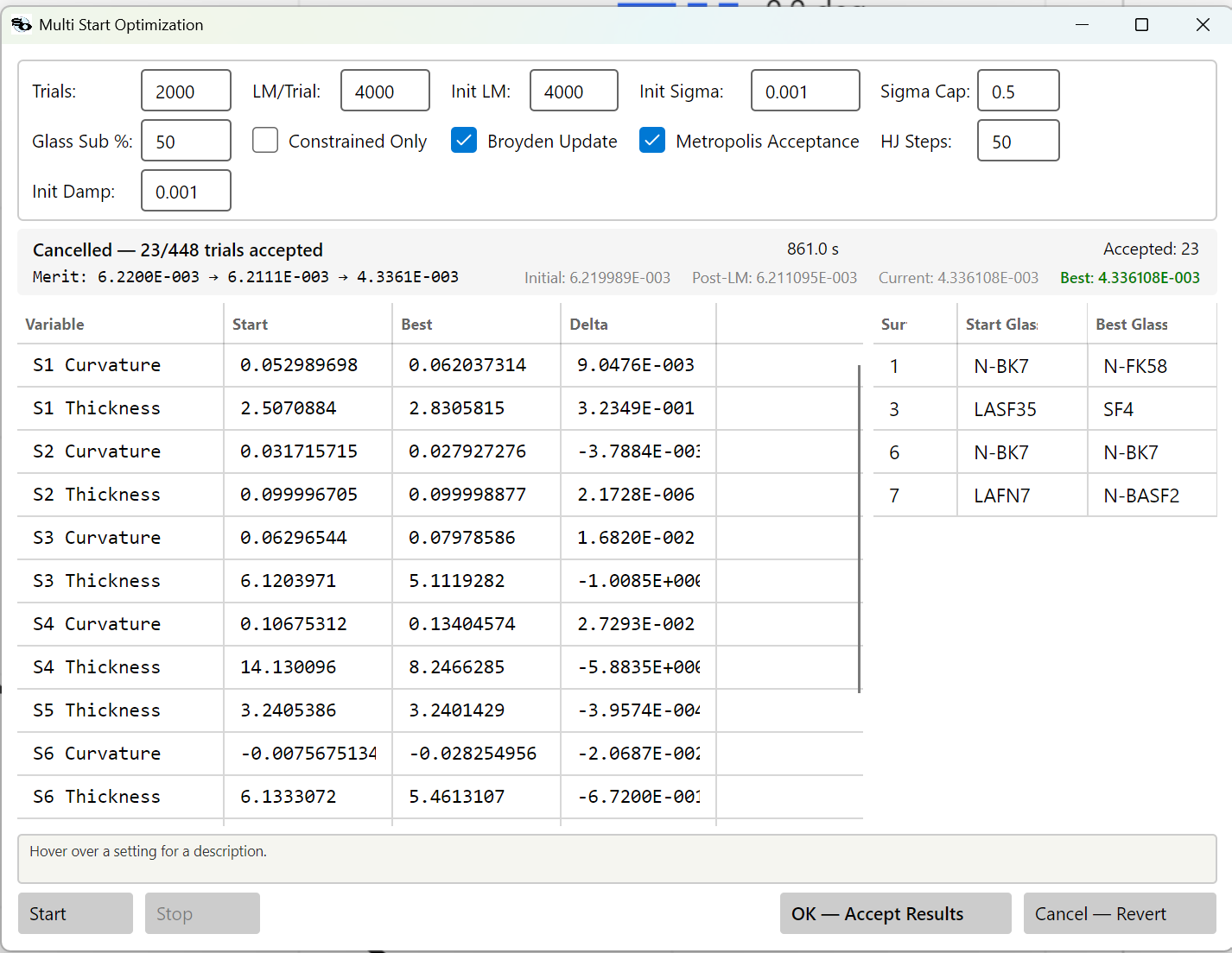
When to reach for SPC:
- The starting design has too few elements for the aberration budget (one or two lenses trying to do an apochromat's job).
- You want the program to discover topology — pre-stop vs post-stop, singlet vs doublet — rather than handing it a fixed surface count to refine.
- You don't already know how many elements the design needs.
Max Elements = 2lets you watch the merit drop level by level and stop when the gains plateau.
What it isn't:
- A polish step. Always finish with Local LM and a Multistart pass with glass substitution. SPC's per-branch glass trials only sample a random subset and its per-branch LM is bounded — enough to rank branches, not to grind out the last percent of merit. The case study above shows Multistart finding ~30 % further improvement on top of the SPC output and shuffling 3 of 4 glass picks; that's typical, not exceptional.
- A short-budget tool when doublets are enabled. "Single +
Cemented Doublet" with
Max Elements = 2and a real catalog takes minutes to tens of minutes per level on a multi-core machine.
Common Workflow
- Load a starting design that already traces. On-axis vignetting is heavily penalized — see Merit Function § Failure handling — so the start needs at least all on-axis pupil rays reaching the image.
- Tag curvatures and airspaces as Variable with physical bounds — typically 1–2 mm minimum on glass, 0.1 mm minimum on air, generous maxima.
- Set up a merit function: a
WAVEXorSPOToperand for image quality, anEFLtarget with high weight (≥ 100), boundary operands (EG/EA/TTRACK) to keep the geometry manufacturable. - Run Local Optimizer first. If merit stops far from where you want, run Multistart (a few hundred trials, ~2 % perturbation, glass substitution on if you have substitution surfaces).
- Still stuck? Run Basin Hopping — defaults plus 100–500 hops, ideally with glass substitution. Stop early when you see the merit has plateaued.
- Always finish with a Local Optimizer pass so the final state is LM-converged.
Stopping an Optimization
Press Stop on the optimizer dialog at any time. The current operation cancels at the next safe point and the best value found so far is kept until you click OK — Accept Results (commits the optimized state) or Cancel — Revert (restores the original).
Performance Tips
- Broyden on, default tolerance. 3–5× faster than a full Jacobian every iteration and matches results in almost all cases.
- Lock the focal length. Adding an
EFLoperand with a tight target (weight ≥ 100) often dramatically stabilizes the search — the optimizer can't "cheat" by shifting focus to hide aberrations. - Bound air thicknesses below. Without an
EAminimum operand or a per-variableMinon each airspace, the optimizer can collapse airspaces to zero or negative values during exploration. - Don't over-vary. Marking every available parameter Variable inflates the dimensionality and makes basins shallower. Start minimal; add more only when the merit plateaus.
- Multistart for glass searches, Basin Hopping for topology. If your topology is already good and you only want to vary glass, Multistart at ~50 % glass-swap probability iterates faster. Basin Hopping is the right tool when the shape of the design is in play.
Glass Catalogs
LensHH-LT represents every glass element with a reference to an entry in a glass catalog. Catalogs are ZEMAX AGF (ASCII glass-file) format. Five manufacturer catalogs ship with the installer; you can add custom catalogs with the Glass Catalog Generator tool.
What Ships
| Catalog | Manufacturer |
|---|---|
| SCHOTT | Schott AG (Germany) |
| OHARA | Ohara Corp. (Japan) |
| HOYA | Hoya Corp. (Japan) |
| SUMITA | Sumita Optical (Japan) |
| CDGM | CDGM Glass (China) |
Files live in <install>\catalogs\Glass\ and are loaded automatically
on startup.
If you maintain custom or filtered catalogs, drop them under
<install>\catalogs\FilteredGlassCatalogues\. Any *.agf file in
either folder is picked up.
How a Glass Is Named
A glass entry is identified by its name (e.g. N-BK7, LAK9,
S-TIH6) plus the catalog it belongs to. A lens file's surface
record typically stores just the name; LensHH-LT resolves it by:
- Exact match on
CATALOG:NAMEif the lens file uses that form. - Otherwise, searching the system's preferred catalog list
(declared on the ZMX
GCATline, or set via File → Catalog Preference…). - Finally, a scan of every loaded catalog.
When two catalogs contain the same name (common — SF5 exists in
SCHOTT and older catalogs), the preferred-catalog order decides which
one wins. Reorder the list via File → Catalog Preference… if the
resolver is picking the wrong one.
Names in Code V files
Code V glass names carry no punctuation. The names above are written
NBK7 and STIH6 in a .seq file, and the same applies to every
vendor: Ohara S-FPL51 is SFPL51, CDGM H-ZF52 is HZF52. Export
strips the punctuation for you.
Import cannot simply reverse that, because the punctuation-free spelling
is genuinely ambiguous — Hoya ships real catalog names like NBFD10
that must be left exactly as they are, while NBK7 has to become
N-BK7. Nothing in the spelling separates the two cases, so import
resolves the name against your loaded catalogs instead of transforming
it: a name that a catalog claims as written is kept, otherwise the entry
whose punctuation-stripped form matches is used. Load your catalogs
before importing a .seq — with none loaded there is nothing to
resolve against, and only the Schott N-prefix is recovered.
The catalog travels with the glass
A bare name does not always identify a glass. SK16 is in both SCHOTT
and SUMITA with the same n_d but different dispersion formulas, so which
one a bare SK16 binds to depends on the order catalogs happen to be
searched in. Stripping punctuation adds collisions of its own: Sumita
P-SK50 and Schott PSK50 both become PSK50.
Export therefore writes the catalog alongside the name, in Code V's
GLASS_CATALOG form — NBK7_SCHOTT, SFPL51_OHARA, SK16_SUMITA — and
import records those catalogs on the system, where they become the
preferred-catalog order for every later lookup.
A qualifier is only written when the owning catalog is one Code V ships:
HOYA, OHARA, SCHOTT, CDGM, SUMITA, HIKARI, CORNING. A glass from a
catalog Code V does not have — MISC, PATENTMODEL, LightPath, or a custom
catalog of your own — is written bare, because naming a catalog Code V
cannot find would make the material unresolvable there. We hold Corning
in two catalogs, CORNING_B and CORNING_FS; both are written as Code
V's single CORNING, and import maps it back.
Where several of your catalogs answer to one name, the system's own catalog preference decides which is written. With no preference set there is nothing to justify a choice, so the name goes out bare.
One spelling cannot survive the trip. A glass whose name genuinely
contains an underscore — ZEMAX's MoldStress extension writes MS_PMMA
— imports correctly, since PMMA is not a catalog name, but exports as
MSPMMA. Code V reads _ as the catalog separator, so there is no way
to write that name in a .seq and have it read back whole.
Status Flags
AGF entries carry a status code that LensHH-LT reads and surfaces in the glass picker:
| Code | Meaning | When to use |
|---|---|---|
| 0 | Standard | Production-ready. Default filter includes these. |
| 1 | Preferred | Manufacturer-recommended. Good default for new designs. |
| 2 | Obsolete | Still characterized but no longer sold. Avoid for new designs. |
| 3 | Special | Low-volume or custom. May be expensive or have long lead times. |
| 4 | Melt | One-off melt data. Only meaningful for as-built analysis. |
The glass-substitution step in the multistart and basin-hopping optimizers can be restricted to any subset of these statuses.
Dispersion Formulas
Each catalog entry carries a formula code and a list of coefficients. LensHH-LT supports:
| Code | Formula | Coefficients |
|---|---|---|
| 1 | Schott | 6 (a0..a5) |
| 2 | Sellmeier 1 | 3 terms (K₁, L₁², K₂, L₂², K₃, L₃²) |
| 3 | Herzberger | 6 (returns n directly) |
| 4 | Sellmeier 2 | 3 terms (B₁, B₂, B₃, B₄, B₅, B₆) |
| 5 | Conrady | 3 (n = a + b/λ + c/λ^3.5) |
| 6 | Sellmeier 3 | 4 terms (K, L² pairs) |
Wavelength is always in micrometers. An entry with no recognized
formula falls back to its Nd value (1.5 if unknown).
Validity Range
Each entry carries WavelengthMin / WavelengthMax lines (AGF
LD ...). LensHH-LT does not automatically refuse wavelengths
outside this range — dispersion formulas extrapolate, and the glass
may not transmit. Check against the manufacturer's transmission chart
when you're using wavelengths far from the visible band.
The Glass Picker
Every glass cell in the Surfaces table opens a picker dialog showing:
- Search box (live-filters by partial name).
- Catalog filter (multi-select).
- Status filter (Standard / Preferred / Obsolete / Special / Melt).
- Column sort for name, catalog, Nd, Vd, status.
- Per-row preview of Nd, Vd, partial dispersion ratios.
Double-click an entry (or press OK) to assign it to the current surface.
Model Glass (Nd / Vd / dPgF)
Instead of a named catalog entry, a surface's glass can be a model glass — a refractive index computed directly from three numbers:
- Nd — refractive index at the d-line (587.6 nm).
- Vd — the Abbe number (dispersion).
- dPgF — the deviation of the relative partial dispersion (Pg,F) from the "normal line", which sets the anomalous dispersion that drives secondary-spectrum correction.
The engine builds a full dispersion curve from these three values, so a model glass behaves like any real glass in ray tracing, analysis, and optimization — but it need not exist in any catalog. That makes it the tool for exploring what glass a design wants before you go shopping for a real one.
Enabling it
Open a surface's Properties → Glass Model tab. Start with a
catalog glass assigned — here surface 3 of a Cooke triplet is F2:
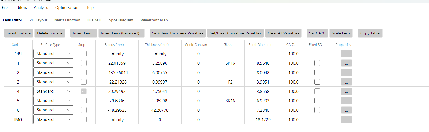
With Enable Model Index off, the Nd/Vd/dPgF fields are disabled and the surface keeps its catalog glass:
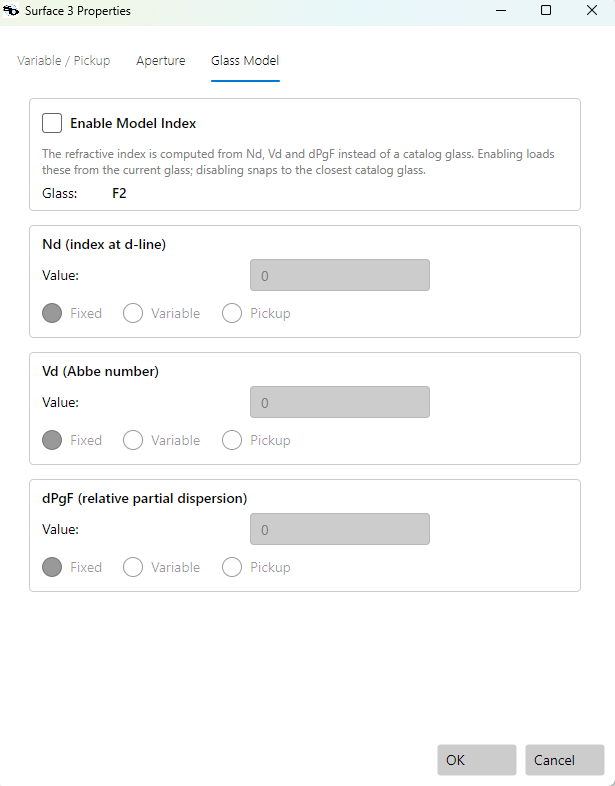
Check Enable Model Index and the three fields populate from the current glass (F2's Nd ≈ 1.6200, Vd ≈ 36.37, dPgF ≈ 0.000279), and the glass label changes to Model:
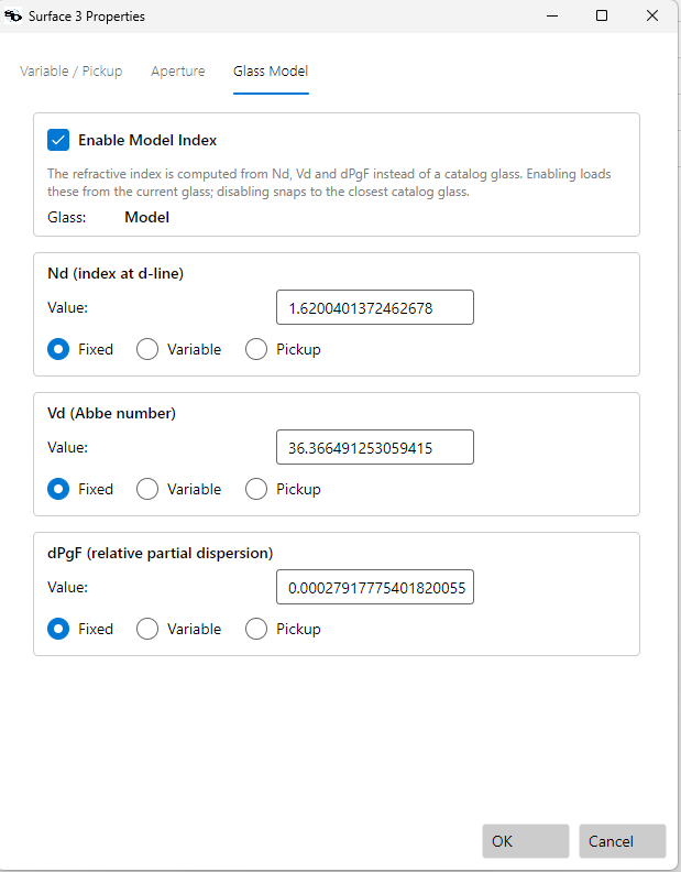
Each parameter carries the familiar Fixed / Variable / Pickup choice, so Nd, Vd, and dPgF can each be optimization variables — letting the optimizer move continuously through index/dispersion space — or pickups slaved to another surface's model. (A pickup source must itself be a model-index surface; the picker only offers those, so a model parameter can never pick up a meaningless 0 from a catalog glass.)
Edit a value directly to explore a hypothetical glass — say Nd = 1.65, higher than F2:
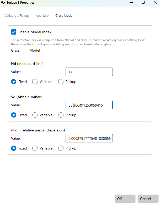
In the Lens Editor the glass column now reads Model for that surface:
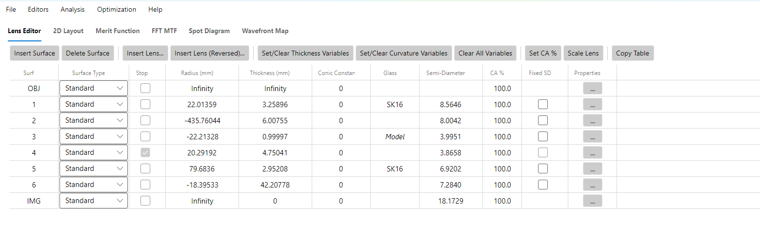
Snapping back to a real glass
When you have a model index you like, uncheck Enable Model Index and the surface snaps to the closest catalog glass — the nearest real glass in Nd/Vd/dPgF space. Because we raised Nd to 1.65, the closest match is no longer F2 but F6:
| Snapped to F6 in the dialog | …and in the Lens Editor |
|---|---|
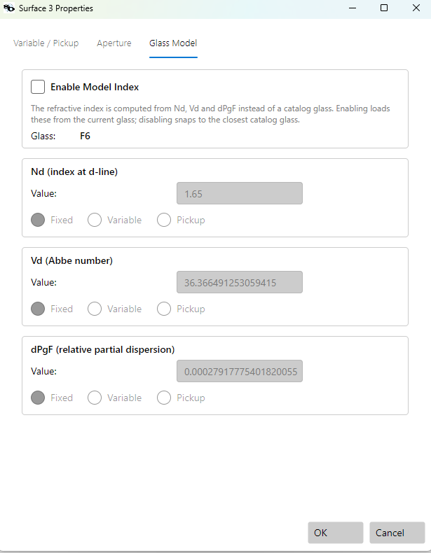 |
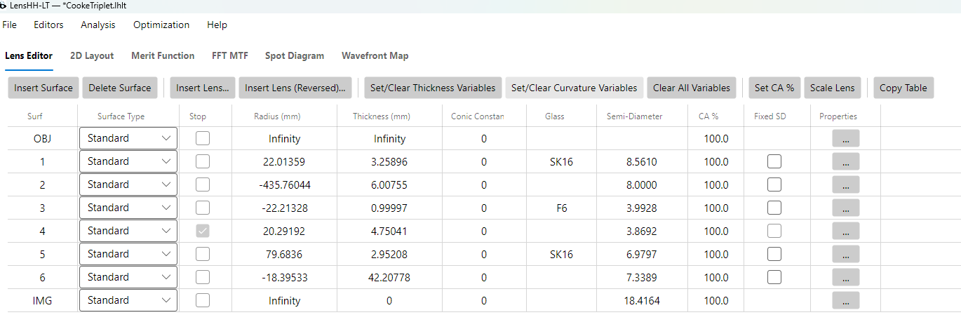 |
The round trip — start from a catalog glass, free Nd/Vd/dPgF as variables, optimize, then snap to the nearest real glass — is a standard way to let a design tell you which glasses it wants before committing to a manufacturable set.
Custom / Filtered Catalogs
Why
A full manufacturer catalog contains 200+ entries, many of which are obsolete, special-order, or outside your wavelength band. For optimization (glass substitution in particular), restricting the search to a curated sub-catalog makes the search both faster and more manufacturable.
How
Optimization → Create Glass Catalogue…
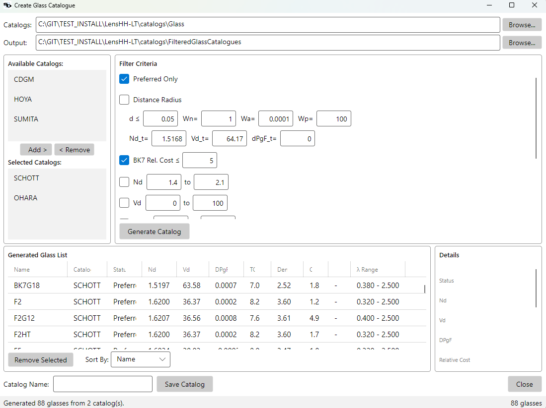
Workflow:
Catalogs / Output paths at the top default to your install's
catalogs\Glassandcatalogs\FilteredGlassCataloguesfolders; change either with Browse… if you want to pull from a non-standard location.Pick source catalogs. The left pane lists every AGF in the Catalogs folder. Use Add > / < Remove to move catalogs between Available and Selected; the survivors are pulled from the union of Selected.
Enable the filters you want. Each filter has a checkbox; only checked filters are applied. The full filter set:
Filter Meaning Preferred Only Status flag ≤ 1 (Standard or Preferred). Drops Obsolete / Special / Melt entries. Distance Radius Multivariate distance from a target glass in (Nd, Vd, ΔPgF) space. d = √(Wn·(Nd − Nd_t)² + Wa·(Vd − Vd_t)² + Wp·(ΔPgF − ΔPgF_t)²). Useful for "glasses near N-BK7" — set the targets to BK7's properties and lowerduntil the count is what you want.BK7 Rel. Cost ≤ Drop entries whose relative-cost factor exceeds this multiple of N-BK7. Nd / Vd / dPgF / TCE ranges Rectangular bounds on each individual property. Min / Max wavelength Keep only glasses with LDvalidity covering this range. Tied to your design band.Melt frequency limit Drop melts characterized fewer than N times — a rough manufacturability proxy. Generate Catalog. The bottom-pane Generated Glass List fills with the surviving entries. Click any row to see its full properties in the Details panel on the right; Remove Selected drops a row by hand if you want to prune further. Sort the list by Name, Nd, Vd, ΔPgF, Relative Cost, or TCE.
Catalog Name + Save Catalog. The dialog writes a fresh AGF file under the Output folder.
Restart LensHH-LT. Filtered catalogs are loaded on startup only — there is no live-reload menu.
A typical starter pool for visible-band designs: Preferred Only
- Min wavelength = 0.42, Max wavelength = 0.7, BK7 Rel. Cost ≤ 5, sources = SCHOTT + OHARA. Yields ~80–120 glasses, which is small enough that Multistart / Basin Hopping can sweep it quickly while still spanning a wide Abbe range.
Cherry-pick from existing catalogs
Optimization → Create Filtered Catalogue (Cherry-_Pick)…
The criteria-based generator is good when you can describe the glasses you want as a set of property bounds. When you'd rather hand-assemble a small catalog — say, "the eight glasses our shop already has on the shelf", or "BK7 plus the four substitutes I trust to swap for it" — the cherry-pick dialog lets you build the catalog one entry at a time from the union of any source catalogs you load.
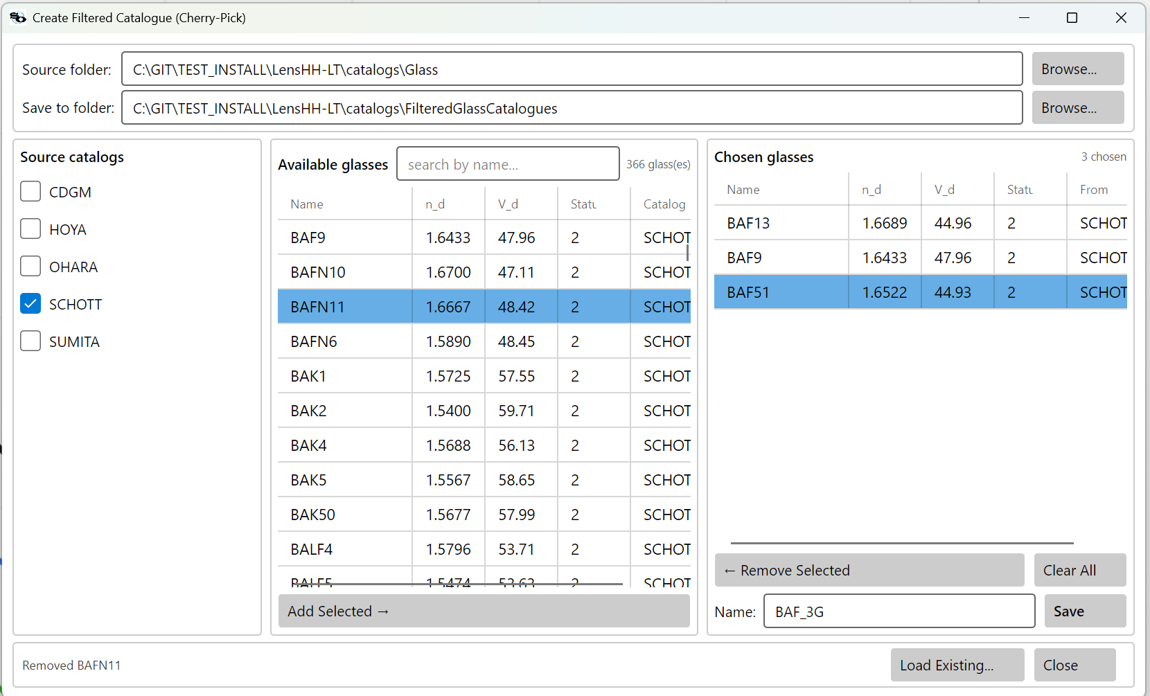
Workflow:
- Source folder / Save to folder at the top default to
your install's
catalogs\Glassandcatalogs\FilteredGlassCataloguesfolders. Change either with Browse… if you want to pull from or save to a non-standard location. - Check the source catalogs in the left pane. The middle Available glasses pane fills with the union of glasses from every checked catalog. The count next to Available glasses updates live; the search by name… box filters the list.
- Add glasses to your catalog. Select rows in Available glasses and click Add Selected →, or double-click a single row. They appear in the right Chosen glasses pane.
- Refine the chosen list with ← Remove Selected (drop one) or Clear All (start over).
- Name it and click Save. The dialog writes a fresh AGF file under the Save to folder with the entries you picked.
- Restart LensHH-LT. Same as the criteria-based catalogs — filtered catalogs load on startup only.
The Load Existing… button at the bottom lets you open an existing filtered AGF as the starting Chosen glasses list, so you can extend or trim a catalog you already have without re-picking everything.
Cherry-picked catalogs work identically to criteria-built ones — both are AGF files in the FilteredGlassCatalogues folder, both appear in the per-surface Glass Substitution dropdown and in the Basin Hopping Glass Source dropdown.
AGF Format Primer
An AGF catalog is plain text. Each glass occupies one block with a handful of tagged lines. LensHH-LT uses three tags:
NM  name formula MIL Nd Vd Exclude Status
CD  c0 c1 c2 c3 c4 c5 ...
LD  wavelength_min wavelength_max
All other lines (GC, TD, OD, IT, …) are permitted in the file
but currently ignored by the reader. This means transmission curves
(IT), thermal coefficients (TD), and relative-cost data (OD) are
not consumed by LensHH-LT — if you need those for a secondary
tool, keep the original manufacturer AGF around.
Example entry:
NM N-BK7 1 517.642 1.51680 64.17 0 1
CD 1.03961212 2.31792344e-1 1.01046945 6.00069867e-3 2.00179144e-2 1.03560653e2
LD 0.3 2.5
Formula code 1 = Schott, 6 coefficients, valid 0.3–2.5 µm.
Glass Substitution During Optimization
Multistart and Basin Hopping both can swap glasses during a search, but they use very different mechanics. Pick the one that matches the level of control you want.
Multistart — per-surface table
Multistart reads a per-surface substitution table that lives on
the system itself (saved in the .lhlt). Each glass surface has its
own opt-in flag and its own catalog choice, so different surfaces
can draw from different filtered catalogs.
To populate the table, open Optimization → Glass Substitution Settings:
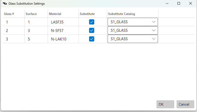
The dialog lists every glass surface in the system. For each row:
- Substitute — tick to opt that surface into substitution.
- Substitute Catalog — pick a filtered catalog from the
dropdown. The dropdown is populated from
<install>\catalogs\FilteredGlassCatalogues\; if it's empty, generate one first via Create Glass Catalogue….
OK writes the choices to the system (and they're persisted in
the .lhlt file). When Multistart runs with
GlassSubstitutionProbability > 0, every trial rolls per-surface:
with probability p, that trial picks a random glass from that
surface's catalog. Surfaces without Substitute = true are never
touched.
Basin Hopping — single shared catalog
Basin Hopping doesn't use the per-surface table at all. Its Glass Source dropdown picks one filtered catalog and applies it to every glass element that has an active element-local variable (curvature/thickness/conic/asphere on either face). Surfaces without active variables are auto-detected and skipped.
See Optimization → Basin Hopping for the full eligibility rules and the run-start log line that reports which elements made the cut.
Choosing a pool
Whatever the mechanism, the pool you point at matters more than either optimizer:
- A full manufacturer AGF (200+ glasses) is too noisy for most searches. Many glasses are obsolete, special-order, or outside your wavelength band; the optimizer wastes hops on them.
- A 30–100-glass filtered catalog (Preferred only, Vd ≥ some cutoff, valid through your wavelength range) typically converges faster and lands on more manufacturable designs.
Use Optimization → Create Glass Catalogue… (described above)
to build filtered catalogs; they're saved automatically to
<install>\catalogs\FilteredGlassCatalogues\ and become available
in the substitution dropdowns after the next app start.
Troubleshooting
| Symptom | Likely cause |
|---|---|
| "Glass 'X' not found" on load | The lens file names a glass that isn't in any loaded catalog. Check catalog-preference order; add the missing AGF. |
| Refractive index looks wrong at short or long wavelengths | Wavelength outside the glass's LD range — dispersion is extrapolated. Use a different glass that's valid at that wavelength. |
| Same glass name resolves to different properties in two lenses | Two catalogs define the name differently (e.g. SF5 in SCHOTT vs. an older vendor). Make the preference order explicit, or reference as CATALOG:NAME. |
| Custom AGF loads but glasses don't appear | Filename must end in .agf (case-insensitive). Contents must start with valid NM blocks — catalog header-only lines without glasses load an empty catalog silently. |
API, CLI, and MCP
Three surfaces let you drive LensHH-LT without the GUI:
- C# API (
LensHH.API,LensHH.Core) — embed or script the engine directly from your own .NET code. - CLI (
LensHH.CLI) — interactive REPL with scripted-input support. - MCP server (
LensHH.Mcp) — exposes the engine as tools for Model Context Protocol hosts (Claude Desktop, Cursor, etc.).
All three share the same OpticalSystem model, MeritFunctionEvaluator,
and optimizer implementations from LensHH.Core, so results are
identical across surfaces.
C# API
The public entry point is LensHH.API.LensHHSession. One session
holds one optical system, its merit function, and a glass catalog
manager. Segregated interfaces let consumers depend on only the
surface they need.
Quick Start
using LensHH.API;
using LensHH.Core.Enums;

var session = new LensHHSession();
session.Initialize();               // load license / trial state

session.ImportZemax(@"C:\lenses\triplet.zmx");
session.SetAperture(ApertureType.EPD, 12.0);
session.SetFieldType(FieldType.ObjectAngle);

// Add a variable for surface 1 curvature:
session.AddVariable(surfaceIndex: 1, parameter: VariableParameter.Curvature);

// Build a minimal merit function:
session.AddMeritOperand(OperandType.SPOT, weight: 1.0);
session.AddMeritOperand(OperandType.EFL, weight: 1.0, target: 100.0);

// Run LM and inspect the result:
var result = session.OptimizeLocal();
Console.WriteLine($"Merit: {result.InitialMerit:E4} → {result.FinalMerit:E4}");

session.SaveAs(@"C:\lenses\triplet-optimized.lhlt");
Object Space NA and object-space telecentric are set the same way (finite conjugate, Object Height fields):
session.SetAperture(ApertureType.ObjectSpaceNA, 0.025);  // NA = n0·sin(u)
session.SetTelecentricObjectSpace(true);                 // EP at infinity; needs NA + ray aiming Off
Segregated Interfaces
LensHHSession implements seven interfaces; you can narrow a
reference to just the capability you need:
| Interface | Purpose |
|---|---|
ILicenseStatus |
Activation state, trial days, machine ID. |
IFileIO |
.lhlt load/save; import/export .zmx, .seq, .len, .otx, .json. |
ISystemEditor |
Mutations: aperture, fields, wavelengths, surfaces, variables, pickups. |
IAnalysis |
Spot diagram, MTF, wavefront, OPD/ray fans, Seidel, Zernike, lateral color, etc. |
IOptimization |
Local LM, Multistart, Basin Hopping, split-element, SPC synthesis. |
IRendering |
Plot/image rendering for GUI consumers (delegates to LensHH.Rendering). |
ITextExport |
Plain-text dumps of analyses for scripting/reports. |
Example of a narrowly-typed consumer:
IAnalysis analysis = session;
var spot = analysis.ComputeSpotDiagram(fieldIndex: 0, waveIndex: -1);
Console.WriteLine($"RMS = {spot.RmsRadius:F4} mm");
Direct LensHH.Core Access
The API sits on top of LensHH.Core. If you need finer-grained
control — say, a custom optimizer that calls MeritFunctionEvaluator
directly — reference LensHH.Core.dll and use:
using LensHH.Core.Glass;
using LensHH.Core.MeritFunction;

var glassMgr = new GlassCatalogManager();
glassMgr.LoadCatalogsFromFolder(@"catalogs\Glass");

var evaluator = new MeritFunctionEvaluator(session.System, glassMgr)
{
    ParallelEvaluation = true,
    AutoSolveSemiDiameters = true
};
double merit = evaluator.Evaluate(session.MeritFunction!);
Key LensHH.Core namespaces:
| Namespace | Contents |
|---|---|
LensHH.Core.Models |
OpticalSystem, Surface, Aperture, Field, Wavelength. |
LensHH.Core.Glass |
GlassCatalogManager, GlassData, AgfReader. |
LensHH.Core.MeritFunction |
MeritFunction, Operand, OperandType, MeritFunctionEvaluator. |
LensHH.Core.Optimization |
LocalOptimizer, BasinHoppingOptimizer, MultistartOptimizer. |
LensHH.Core.Analysis |
SpotDiagram, FftMtf, WavefrontMap, SeidelCoefficients, etc. |
LensHH.Core.RayTrace |
ArbitraryRay, ParaxialRayTracer, TracerBuffers. |
LensHH.Core.IO |
.lhlt/.zmx/.seq/.len/.otx/.json readers and writers. |
License Gating
Every expensive operation (ray trace, optimization) goes through an
activation check before running. An unlicensed and expired install
throws InvalidOperationException. Call
session.Initialize() once at startup to load the persisted license;
session.Activate(key) or session.ActivateOffline(tokenPath) for
first-time setup.
CLI
Executable: <install>\cli\LensHH.CLI.exe (Windows) or
LensHH.CLI (Linux/macOS).
An interactive REPL. Start with no arguments for an interactive
prompt, or pass --script <file> to run a batch of commands.
Top-Level Commands
| Command | Purpose |
|---|---|
file |
Open, save, import (.zmx, .seq, .len, .otx), export. |
system |
System-level edits — aperture (EPD / FNumber / Object Space NA), field type, wavelengths, ray aiming, afocal & object-space-telecentric flags. |
surface |
Add, remove, insert, edit surfaces; manage aspheric coefficients. |
glass |
Search, load catalogs, show glass properties, generate filtered catalogs. |
pickup |
Surface-to-surface parameter pickups. |
var |
Mark parameters as variables with optional bounds. |
merit |
Build and evaluate the merit function. |
optimize |
Run Local LM, Multistart, Global Search (optimize global), Basin Hopping, Global Basin Hopping, Split Element, SPC or DE — and optimize preview, which reports which engine a run would use without running it. |
analysis |
Run any analysis (spot, mtf, wavefront, seidel, etc.) and print results. |
log |
Control log verbosity and output redirection. |
script |
Execute a file of CLI commands. |
shell |
Shell-out to the host OS. |
license |
Show license status, activate online or with a token file. |
Every command auto-completes sub-verbs and parameters. Type the
command alone (e.g. merit + Enter) for context help.
Scripting
Commands accept the same arguments whether typed interactively or
loaded via --script. Example script:
# triplet-opt.lhscript
file import triplet.zmx
system aperture epd 12
system wavelength add 0.486
system wavelength add 0.656
var add 1 curvature
var add 2 curvature
var add 3 thickness
merit add spot weight=1
merit add efl target=100 weight=1
optimize local iterations=50
file save-as triplet-optimized.lhlt
analysis spot --field 0 --wave -1
Run with:
LensHH.CLI --script triplet-opt.lhscript
Object Space NA & object-space telecentric (finite-conjugate, Object Height):
system set-aperture na 0.025        # NA = n0·sin(u); also 'epd' / 'fno'
system set-telecentric on           # requires the NA aperture + ray aiming Off
system info                         # shows Aperture, Field Type, Telecentric Object Space
system set-telecentric on is rejected (with a message) unless the aperture is
Object Space NA and ray aiming is Off. See
System Aperture & Object-Space Telecentric.
Bound handling and a reproducible Multistart (new in 1.0.147):
system set-bound-handling reflect   # or sigmoid (default); system info shows it
optimize multistart trials=500 seed=1
optimize multistart trials=500 seed=2   # an independent run, same settings
Bound handling is a system-level setting saved in .lhlt, so it travels with the
design. The Multistart seed defaults to 1 — a run repeats exactly unless you
change it. See Bound handling.
Paraxial (ideal thin lens) surfaces. Set a surface to an ideal lens by giving it a focal length, then optimise its power (diopters):
surface edit 2 focal-length=75          # makes surface 2 Paraxial, f = 75 mm
surface variable focal-length 2 on min=8 max=15   # vary it; bounds are DIOPTERS (1000/f)
var list                                # shows "Focal Power  13.3333 D (f=75 mm)"
The MCP server exposes the same via edit_surface (property="type" →
paraxial, or property="focal_length") and set_variable
(property="focal_power", min/max in diopters); the C# API adds
SetSurface(..., focalLength:) and SetFocalLengthVariable(index, minPower, maxPower).
Which engine will this run use? (new in 1.0.152)
optimize preview answers the same question the GUI's Preview button does,
and asks the same code the optimizer uses to choose, so it cannot disagree with
the run:
file open design.lhlt
optimize preview                        # as the optimizer would run it
optimize preview engine=csharp          # what a C# run would look like
optimize preview analytic=false         # native, finite-difference
optimize preview broyden=false          # PSD's default; changes the answer
optimize preview gpuimage               # include the GPU image-quality path
WILL RUN:  C# Finite-Difference (fell back from Native: model-glass variables)

Requested: Native Analytic

DOWNGRADED, because:
  model-glass variables

Also:
  - Native engine: loaded (v0.1.0).
  - 21 variable(s), 27 merit operand(s).
  - GPU: not requested - the merit runs on the CPU.
broyden= matters more than it looks: it defaults to on for LM and off for the
PSD steps, and some fallbacks depend on it. If a PSD run is slower than the same
design under LM, preview both and compare.
Choosing the engine explicitly (new in 1.0.152):
optimize run maxiter=200 engine=csharp analytic=false
optimize basin hops=200 engine=native analytic=true
optimize multistart trials=200 engine=native
optimize global-basin globalmin=30 engine=native
engine=native|csharp and analytic=true|false are accepted by run,
multistart, basin, global-basin and global. All of them default to
native + analytic, matching the GUI dialogs; before 1.0.152 the CLI defaulted
to C# finite-difference while the dialogs did not, so the same run took a
different path depending on where you launched it.
The optimizer still falls back on its own when a design needs it — the flags
express a preference, and optimize preview tells you what survived.
Reseeding a stalled chain (new in 1.0.152):
optimize basin hops=1000 chains=0 elitehops=150 elitefactor=10
optimize basin hops=1000 elitehops=0                 # rescue off
optimize global-basin globalmin=60 elitehops=150 elitefactor=3
A chain is handed another chain's best design only when it has gone
elitehops hops with no best of its own and its own best is worse than
elitefactor × the best design found so far. Both are required: the hop count
alone is not a stall, and acting on it alone collapses every chain onto the
leader. elitehops=0 disables it. See
Reseeding a chain that has fallen behind
for how to choose the factor.
Diagnosing a local-optimizer stall. Set LENSHH_LM_DEBUG to a file path and
every LM iteration — accept/reject, damping, step and gradient norms — is
appended to it, for every subcommand including the inner LM of a basin hop:
LENSHH_LM_DEBUG=lm.log LensHH.CLI --script run.lhscript
Exit Codes
The CLI returns a non-zero exit code when a command fails or a script
aborts. Useful for CI/batch automation: LensHH.CLI --script foo.txt || exit 1.
MCP Server
Executable: <install>\mcp\LensHH.Mcp.exe (Windows) or
LensHH.Mcp (Linux/macOS).
A Model Context Protocol server that exposes the engine as tools an LLM can invoke. Uses standard stdio transport per MCP spec.
Configuring Claude Desktop and Claude Code
LensHH-LT ships a small Windows utility — Start Menu → LensHH-LT
Claude Configure — that registers (or unregisters) the MCP server
with both Claude clients in one place. It auto-detects the bundled
LensHH.Mcp.exe; a green check appears once the path resolves.
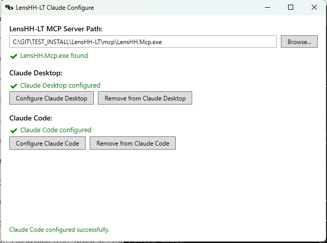
| Section | Configure button | What it does | Remove button |
|---|---|---|---|
| Claude Desktop | Edits %APPDATA%\Claude\claude_desktop_config.json, adding an mcpServers.LensHH-LT entry that points at the MCP exe. |
Reverts the edit. | Restart Claude Desktop for the change to take effect. |
| Claude Code | Shells out to claude mcp add --transport stdio --scope user LensHH-LT -- "<exe>", so the registration goes through the official Claude Code CLI. If claude isn't on PATH the equivalent command is copied to your clipboard. |
Runs claude mcp remove --scope user LensHH-LT. |
Status indicators below each section show whether the registration is currently active, so you can use the same utility to verify the setup after install or after moving the install path.
Manual configuration (Claude Desktop, if you prefer to edit JSON by hand):
{
  "mcpServers": {
    "LensHH-LT": {
      "command": "C:\\Program Files\\LensHH-LT\\mcp\\LensHH.Mcp.exe",
      "args": []
    }
  }
}
Manual configuration for Claude Code (the utility runs this verbatim):
claude mcp add --transport stdio --scope user LensHH-LT -- "C:\Program Files\LensHH-LT\mcp\LensHH.Mcp.exe"
Other MCP-aware hosts (Cursor, custom clients) use the same exe/args as the Claude Desktop JSON block.
Claude Code vs Claude Desktop — which to use
Both clients can drive every tool in the server, but they handle long-running tools very differently. Claude Code is the recommended host for any optimization that runs for more than a minute. Specifically:
- Multistart Optimization
- Global Search
- Basin Hopping (HJ-LM)
- Split Element
- Synthesis by SPC
These five are not exposed as single blocking calls. They run as
background jobs: a *_start tool kicks the work off on a worker
thread and returns immediately with a jobId. The host then polls
optimize_status(jobId) for progress (phase, current trial / hop /
level, accepted vs rejected, current best merit, elapsed time) and
calls optimize_cancel(jobId) to stop early. optimize_jobs lists
every job tracked by the current session.
| Tool | Returns | Used to … |
|---|---|---|
optimize_multistart_start |
jobId | Start the optimizer in the background |
optimize_global_search_start |
jobId | Same — Global Search (gallery of distinct design forms); reproducible from baseSeed |
optimize_basin_hopping_start |
jobId | Same — BH variant |
optimize_split_element_start |
jobId | Same — Split Element variant |
optimize_synthesis_by_spc_start |
jobId | Same — SPC variant |
optimize_status |
progress fields | Poll a running job |
optimize_cancel |
confirmation | Request cancellation |
optimize_jobs |
one row per job | List every job tracked by the session |
The job pattern exists because these optimizers routinely run for many minutes (Multistart) to many hours (SPC, Split Element). Claude Code is a much better fit for this:
- It maintains a long-lived session and is comfortable polling on a 10–30 second cadence over hours.
- It can be left to drive the optimization unattended.
- Its result-rendering doesn't share Claude Desktop's per-turn output / response-time constraints, which can stall on tool calls that emit lots of incremental progress.
Claude Desktop is fine for short interactive tool calls
(spot_diagram, fft_mtf_vs_freq, single optimize_local runs,
analyses in general). For the four long-running optimizers above,
use Claude Code — register both with the utility shown above and
pick the right one for the task at hand.
Tool Categories
All tools operate on a single implicit session (McpSession) shared
across the server process. Loading a new system replaces the one in
the session. The ~174 tools group as:
| Category | Tool count | Examples |
|---|---|---|
System (SystemTools) |
28 | system_new, system_load, system_save, system_import_zmx, system_set_aperture (type EPD / FNumber / ObjectSpaceNA), system_set_telecentric_object_space, system_set_wavelengths, system_set_fields, system_set_bound_handling (Sigmoid / Reflect), system_get_info. |
Surface (SurfaceTools) |
11 | surface_add, surface_insert, surface_remove, surface_set, surface_list, surface_set_asphere. |
Glass (GlassTools) |
11 | glass_load_catalogs, glass_list_catalogs, glass_search, glass_get_info, glass_get_index, glass_set_substitution, glass_generate_filtered_catalog. |
Pickup (PickupTools) |
5 | pickup_add, pickup_remove, pickup_list, pickup_clear. |
Optimization (OptimizationTools) |
28 | merit_add_operand, merit_list, merit_edit_operand, merit_evaluate, variable_add, variable_list, optimize_local, optimize_multistart_start, optimize_global_search_start, optimize_basin_hopping_start, optimize_status. |
Analysis (AnalysisTools) |
22 | trace_ray, spot_diagram, ray_fan, pupil_aberration_fan, opd_fan, seidel, wavefront_map, fft_psf, fft_mtf_vs_freq/vs_field/through_focus, geo_mtf_*, zernike_standard, zernike_fringe, lateral_color, relative_illumination, chromatic_focal_shift, field_curvature_distortion. |
Rendering (RenderingTools) |
45 | render_analysis_png, render_layout_png, and per-analysis text-export tools (one analysis_name_text tool per analysis). |
Stock lenses (StockLensTools) |
6 | search_stock_lenses, insert_stock_lens, find_matching_stock, replace_element. |
Batch design search (BatchDesignSearchTools) |
6 | batch_design_search_start, batch_design_search_status, batch_design_search_keep. |
Sasian design (SasianDesignTools) |
5 | sasian_design_start, sasian_design_status, sasian_design_discard. |
DE pipeline (DePipelineTools) |
5 | de_pipeline_start, de_pipeline_status, de_pipeline_discard. |
License (LicenseTools) |
2 | license_status — shows activation/trial state. |
Total: ~174 tools.
Every tool has an [McpServerTool, Description(...)] attribute with a
plain-English description of what it does and what each parameter
means. An LLM discovering the server via MCP's introspection will see
those descriptions verbatim.
Basin-hopping reseed parameters (new in 1.0.152)
basin_hopping_start and global_basin_hopping_start accept
eliteRestartHops (default 150) and eliteRestartMeritFactor (default 10).
They gate the same rescue the GUI and CLI expose: a chain is handed another
chain's best design only when it has gone that many hops without a best of its
own and its own best is worse than that multiple of the best found so far.
Both conditions are required, and eliteRestartHops = 0 disables the rescue.
If your chains typically finish within a factor of two of each other, a factor of 10 never fires — read the per-chain merits back and set it below the spread you actually observe.
Typical LLM Workflow
With LensHH-LT registered in Claude Desktop or Claude Code, a conversation like this works end-to-end:
User: Open
triplet.zmxinC:\lenses\, add SPOT and EFL=100 merit operands, make all curvatures variable, and run the LM optimizer.
The LLM issues: system_import_zmx, variable_add × 3,
merit_add_operand × 2, optimize_local, then system_get_info to
report back the final merit and surface data.
The rendering tools (render_analysis_png and friends) produce PNG
files the LLM can hand back to the user. Text-export tools produce
machine-readable CSV/text blocks the LLM can quote in its reply.
Rendering Sub-Process
Plot rendering requires Skia, which in turn depends on the Avalonia
GPU bindings. Rather than pulling all of Avalonia into the MCP
server's memory space, the MCP server shells out to
<install>\LensHH.RenderApp.exe for PNG generation. This keeps the
MCP process lightweight (~50 MB) and means the RenderApp is only
launched on demand.
Using a Local LLM (Ollama Bridge)
The MCP server is host-agnostic, but Claude Desktop and Cursor are
cloud-hosted. If you want to drive LensHH-LT from a local LLM —
no API key, no data leaving the machine — use the bundled
LensHH.OllamaBridge. It connects a tool-calling Ollama model to
the MCP server and runs an interactive REPL in your terminal.
Prerequisites
- Install Ollama and start it:
ollama serve - Pull a model that supports tool calling. Recommended starting
points (any will work; bigger = better tool-call accuracy but
slower):
ollama pull qwen3:8b
ollama pull llama3.1:8b
ollama pull mistral-nemo
The bridge itself ships with the LensHH-LT installer — no source build required. (Both the bridge and the MCP server it talks to are already on disk after install.)
Launching
Installed (Windows): Start Menu → LensHH-LT → Ollama Bridge (Local LLM). Or run directly:
"%ProgramFiles%\LensHH-LT\ollama\LensHH.OllamaBridge.exe"
Source build (any OS): from the repo root,
# Windows
launch-ollama-bridge.bat

# Linux / macOS
./launch-ollama-bridge.sh
Or, equivalently:
dotnet run --project src/LensHH.OllamaBridge [mcp-server-path] [model-name]
Both arguments are optional. If omitted, the bridge probes standard
locations for LensHH.Mcp (installed sibling mcp\ folder, or the
project's build output if you're running from source) and prompts
you to pick a model from the list returned by Ollama.
Environment Variables
| Variable | Default | Purpose |
|---|---|---|
OLLAMA_URL |
http://localhost:11434 |
Ollama API endpoint. |
OLLAMA_MODEL |
(prompted if unset) | Skip the model-selection prompt. |
OLLAMA_TEMP |
0.1 |
Sampling temperature. Low values keep tool-call JSON well-formed. |
OLLAMA_NUM_CTX |
8192 |
Context window. Raise it (e.g. 32768) for long sessions; the model must support it. |
OLLAMA_STREAM |
true |
Stream tokens as they arrive. Set to false for a single-block response. |
LENSHH_MCP_PATH |
(auto-discovered) | Absolute path to LensHH.Mcp.exe/.dll if it isn't in a standard location. |
Example — pin a model and raise the context window:
# Linux / macOS
OLLAMA_MODEL=qwen3:14b OLLAMA_NUM_CTX=32768 ./launch-ollama-bridge.sh

# Windows (PowerShell)
$env:OLLAMA_MODEL="qwen3:14b"; $env:OLLAMA_NUM_CTX="32768"; .\launch-ollama-bridge.bat
REPL Commands
Inside the prompt, type:
- A natural-language request — the model decides which MCP tools to
call. Tool calls are echoed as
[Tool: tool_name]with a truncated result preview; the full result is fed back to the model. tools— list every MCP tool the bridge discovered.quitorexit— shut down (also closes the MCP subprocess).
Example Session
You> Open C:\lenses\triplet.zmx, set the EPD to 12 mm, and tell me the EFL.
  [Tool: system_import_zmx]
  {"ok":true,"surfaces":5}
  [Tool: system_set_aperture]
  {"ok":true}
  [Tool: system_get_info]
  {"efl":99.83,"bfl":94.21,"track":108.4,...}
LensHH> Loaded triplet.zmx (5 surfaces) and set EPD = 12 mm.
        Effective focal length is 99.83 mm.
Choosing a Model
Tool-calling quality matters more than raw size. As of this writing:
qwen3:8b— solid baseline, fast, reliable JSON.qwen3:14b/qwen3:32b— more accurate multi-step plans.llama3.1:8b— comparable toqwen3:8b; sometimes better at free-form explanation.mistral-nemo— fast on modest hardware; occasional malformed-tool-call retries.
Avoid models without explicit tool-call training (most pre-Llama-3.1 checkpoints) — they will either ignore the tools or emit JSON that fails to parse.
Troubleshooting
Cannot connect to Ollama— make sureollama serveis running; checkOLLAMA_URLif Ollama is on a different host or port.LensHH.Mcp server not found— buildLensHH.Mcpfirst, or setLENSHH_MCP_PATHto the full path of the executable/dll.- Tool calls keep failing with parse errors — the model is too
small or not tool-call trained. Try
qwen3:8bor larger, lowerOLLAMA_TEMPfurther (e.g.0.0), and rerun. No models found— pull at least one model withollama pull <name>.
Writing Custom MCP Clients
The MCP server speaks standard MCP over stdio. Any MCP-compliant client can drive it. If you're writing your own client:
- Launch
LensHH.Mcp.exeas a subprocess. - Use MCP introspection (
tools/list) to enumerate tool schemas. - Call tools with
tools/call; the response body is JSON. - Shut down by closing stdin or killing the process.
When to Use Which
| Use case | Best choice |
|---|---|
| Embed the engine in a .NET GUI or service. | C# API — direct, typed, no IPC overhead. |
| Batch-run many designs in CI / nightly jobs. | CLI with --script. |
| Interactive exploration at a terminal. | CLI REPL. |
| LLM-assisted design ("ask Claude to tune this triplet"). | MCP server with Claude Desktop / Cursor. |
| Local LLM-assisted design (no cloud, no API key). | MCP server via the Ollama Bridge. |
| Cross-language driver (Python, Node, etc.) that doesn't want to embed .NET. | CLI via subprocess, or MCP if the client supports it. |
All three share LensHH.Core, so any workflow you prototype in one
translates directly to the others.